How does memorization affect l2?

Black: Agent generated; Red: Added by human

Introduction

How does memorization affect model’s \(\ell_2\) norm? A baseline expectation is that the more a model memorizes, the larger \(\ell_2\) is, because \(\ell_2\) is a reasonable complexity metric of a model (especially when normalization layers are absent). In this blog, using a random dataset, and train an MLP to memorize it, we find a non-monotonic behavior when the model is tasked with memorizing data – \(\ell_2\) first increases, and then decreases as data size increases.

Experimental setup

Dataset: A memorization-style classification benchmark: continuous inputs and class labels are drawn independently, so the task measures raw capacity rather than a smooth input→label rule. Input dimension 9, 17 classes, 100 training and 80 test examples; input law standard_normal, label law uniform_class_probs (shape parameter 1 where it applies). Seed 9266.

More about this dataset: Memorization benchmark dataset: draw random continuous inputs \(x\in\mathbb{R}^{d_{\mathrm{in}}}\), then sample class labels independently of \(x\). Output classes follow a configurable prior: uniform: \(P(c_n)=1/d_{\mathrm{out}}\) power law: \(P(c_n)\propto 1/n^{\alpha}\) exponential: \(P(c_n)\propto e^{-\alpha n}\) Use cross_entropy_loss with this node (the trainer rejects mse_loss here). Cross-entropy measures pure memorization capacity.

Model: The learner is a fully-connected MLP with 2 hidden layers with 100 units each, relu nonlinearities, and init seed 1207. Input and output widths are whatever this block is configured to accept and produce in this run.

Optimizer: We optimize with Adam using learning rate 0.001, momentum decay β₁ = 0.9, variance decay β₂ = 0.999, and numerical floor ε = 1e-08 (the usual Adam defaults unless you changed them).

Loss: The objective is average cross-entropy over the supervised targets (classification / next-token), optionally scaled by 1.

Observables logged during training: Accuracy observable: tracks supervised prediction accuracy (top-1 style) on the batches used during training.

Weight L2 observable: logs the L2 norm of model parameters during training (overall weight vector magnitude).

Trainer: Training runs for 1000 optimizer steps, writing scalars to disk every 10 steps so we can plot curves. Each step updates the model using the chosen dataset, optimizer, and loss; any optional observables are logged on the same schedule.

Base experiment — training and observables

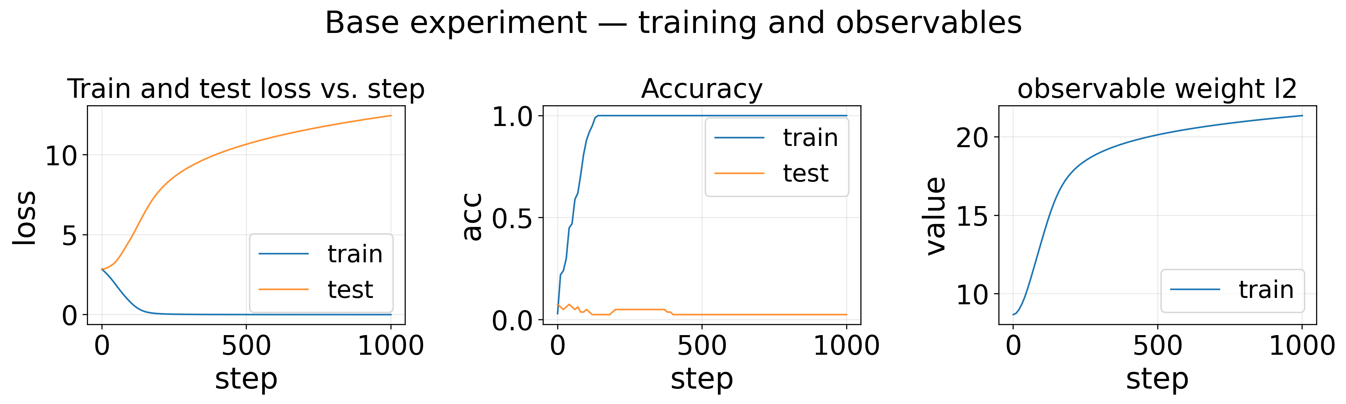
What this strip shows (left → right): each panel is one signal we saved during training; the horizontal axis inside a panel is always the training step unless noted in the title.

Train and test loss vs. step plots training loss on the vertical axis versus optimizer step on the horizontal axis, showing train and (when available) test curves.
Accuracy tracks a logged scalar (train and optional test) versus optimizer step.
observable weight l2 tracks a logged scalar (train and optional test) versus optimizer step.

Note that since it’s a random dataset, it’s impossible to generalize, so it’s expected that test accuracy remains low (random guess) and test loss grows high.

Sweep experiments

Sweep: train size = test size 50, 100, 200, 400, 800, 1600, 3200, 6400, 12800, 25600

Sweep: train size = test size — W_gap_1 — vs sweep parameter (last train step)

What this figure shows: Sweep: train size = test size — W_gap_1 — vs sweep parameter (last train step). It compares the derived scalar metric across sweep “Sweep: train size = test size” as train size = test size changes. How “W_gap_1” is defined: A tensor slice step reduces the upstream tensor by fixing axis 0 at indices 0, producing scalars for the next stage.

Input mapping: \(x_1\) = the 0th value of weight l2 training series; \(x_2\) = the last value of weight l2 training series.

A basic calculator combines those scalars with the rule:

\[x_2 - x_1\]

(The agent still says bullshit sometimes. The gap is simply last-step \(\ell_2\) minus first-step \(\ell_2\).)

Observed phenomena (from the selections in the blog export):

inverted u-shape (train size = test size 50–25600): Inverted-U with maximum near train size 3200 (height 25.763 ≈ 13.5σ). Note that the MLP models roughly has 10000 parameters, if one parameter can memorize 2 bits, and each example requires \(\mathrm{log}(V)\approx 4.1\) bits, the model can memorize rougly \(10000 * 2 / 4.1\approx 5000\) examples, which is the same order as 3200. So one hypothesis is that \(\ell_2\) is maximized when the training size matches model capacity. When data size is small, memorization is easy and the model weight doesn’t need to move much. When data size is large, memorization is hard due to conflicting gradients. This might also be the reason why learning rate warmup is preferred in LLM case (a lot of gradient conflicts in the beginning).
power law (0.27) (train size = test size 50–1600): Curve is monotonic; power-law fit over steps 50–1600 (early (~60% of points); 6 points) with R²=1.000 (A=6.500, B=0.270, C=-9.636).

Code

Code can be downloaded here.