Example 2: Deep Formulas

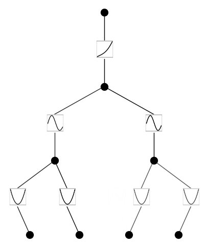
The orignal Kolmogorov-Arnold theorem says that it suffices to have 2-Layer function composition (inner and outer functions), but the functions might be non-smooth or even fractal. We generalize KA representation to arbitrary depths. An example a 2-Layer KAN (with smooth activations) is unable to do is: \(f(x_1,x_2,x_3,x_4)={\rm exp}({\rm sin}(x_1^2+x_2^2)+{\rm sin}(x_3^2+x_4^2))\), which requires at least 3-Layer KANs.

Three-layer KAN

from kan import KAN, create_dataset
import torch

# create a KAN: 2D inputs, 1D output, and 5 hidden neurons. cubic spline (k=3), 5 grid intervals (grid=5).
model = KAN(width=[4,2,1,1], grid=3, k=3, seed=0)
f = lambda x: torch.exp((torch.sin(torch.pi*(x[:,[0]]**2+x[:,[1]]**2))+torch.sin(torch.pi*(x[:,[2]]**2+x[:,[3]]**2)))/2)
dataset = create_dataset(f, n_var=4, train_num=3000)

# train the model
model.train(dataset, opt="LBFGS", steps=20, lamb=0.001, lamb_entropy=2.);

train loss: 1.26e-02 | test loss: 1.20e-02 | reg: 6.73e+00 : 100%|██| 20/20 [00:32<00:00,  1.63s/it]

model.plot(beta=10)

# it seems that removing edge manually does not change results too much. We include both for completeness.
remove_edge = True

if remove_edge == True:
    model.remove_edge(0,0,1)
    model.remove_edge(0,1,1)
    model.remove_edge(0,2,0)
    model.remove_edge(0,3,0)
else:
    pass

grids = [3,5,10,20,50]
#grids = [5]

train_rmse = []
test_rmse = []

for i in range(len(grids)):
    model = KAN(width=[4,2,1,1], grid=grids[i], k=3, seed=0).initialize_from_another_model(model, dataset['train_input'])
    results = model.train(dataset, opt="LBFGS", steps=50, stop_grid_update_step=30);
    train_rmse.append(results['train_loss'][-1].item())
    test_rmse.append(results['test_loss'][-1].item())

train loss: 4.77e-03 | test loss: 4.57e-03 | reg: 7.07e+00 : 100%|██| 50/50 [00:42<00:00,  1.19it/s]
train loss: 1.78e-03 | test loss: 1.84e-03 | reg: 7.15e+00 : 100%|██| 50/50 [00:46<00:00,  1.07it/s]
train loss: 1.56e-04 | test loss: 1.47e-04 | reg: 7.04e+00 : 100%|██| 50/50 [01:10<00:00,  1.41s/it]
train loss: 1.13e-05 | test loss: 1.05e-05 | reg: 7.05e+00 : 100%|██| 50/50 [01:27<00:00,  1.74s/it]
train loss: 6.00e-07 | test loss: 5.07e-07 | reg: 7.05e+00 : 100%|██| 50/50 [01:50<00:00,  2.21s/it]

import numpy as np
import matplotlib.pyplot as plt

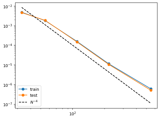
n_params = np.array(grids) * (4*2+2*1+1*1)
plt.plot(n_params, train_rmse, marker="o")
plt.plot(n_params, test_rmse, marker="o")
plt.plot(n_params, 10000*n_params**(-4.), color="black", ls="--")
plt.legend(['train', 'test', r'$N^{-4}$'], loc="lower left")
plt.xscale('log')
plt.yscale('log')
print(train_rmse)
print(test_rmse)

[0.004774762578012783, 0.0017847731212278354, 0.00015569770964015761, 1.1261090479694874e-05, 5.997260680598509e-07]
[0.004566344580739028, 0.0018364543204432066, 0.00014685209697567987, 1.0454170453671914e-05, 5.074556425958742e-07]

Two-layer KAN

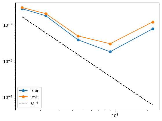
Now we show that a 2 two-layer KAN performs much worse for this task

from kan import KAN, create_dataset
import torch

# create a KAN: 2D inputs, 1D output, and 5 hidden neurons. cubic spline (k=3), 5 grid intervals (grid=5).
model = KAN(width=[4,9,1], grid=3, k=3, seed=0)
f = lambda x: torch.exp((torch.sin(torch.pi*(x[:,[0]]**2+x[:,[1]]**2))+torch.sin(torch.pi*(x[:,[2]]**2+x[:,[3]]**2)))/2)
dataset = create_dataset(f, n_var=4, train_num=3000)

# train the model
model.train(dataset, opt="LBFGS", steps=20, lamb=0.001, lamb_entropy=2.);

train loss: 7.41e-02 | test loss: 7.32e-02 | reg: 1.36e+01 : 100%|██| 20/20 [00:34<00:00,  1.74s/it]

grids = [3,5,10,20,50]
#grids = [5]

train_rmse = []
test_rmse = []

for i in range(len(grids)):
    model = KAN(width=[4,9,1], grid=grids[i], k=3, seed=0).initialize_from_another_model(model, dataset['train_input'])
    results = model.train(dataset, opt="LBFGS", steps=50, stop_grid_update_step=30);
    train_rmse.append(results['train_loss'][-1].item())
    test_rmse.append(results['test_loss'][-1].item())

train loss: 2.75e-02 | test loss: 2.97e-02 | reg: 1.81e+01 : 100%|██| 50/50 [01:24<00:00,  1.69s/it]
train loss: 1.76e-02 | test loss: 2.01e-02 | reg: 1.76e+01 : 100%|██| 50/50 [01:38<00:00,  1.97s/it]
train loss: 3.79e-03 | test loss: 4.85e-03 | reg: 1.78e+01 : 100%|██| 50/50 [01:48<00:00,  2.16s/it]
train loss: 1.77e-03 | test loss: 2.95e-03 | reg: 1.77e+01 : 100%|██| 50/50 [02:07<00:00,  2.55s/it]
train loss: 7.62e-03 | test loss: 1.18e-02 | reg: 1.74e+01 : 100%|██| 50/50 [03:06<00:00,  3.73s/it]

import numpy as np
import matplotlib.pyplot as plt

n_params = np.array(grids) * (4*9+9*1)
plt.plot(n_params, train_rmse, marker="o")
plt.plot(n_params, test_rmse, marker="o")
plt.plot(n_params, 300*n_params**(-2.), color="black", ls="--")
plt.legend(['train', 'test', r'$N^{-4}$'], loc="lower left")
plt.xscale('log')
plt.yscale('log')
print(train_rmse)
print(test_rmse)

[0.027514415570597788, 0.0175788804953916, 0.0037939843087960545, 0.001766220055347071, 0.007622899974849284]
[0.029668332328004216, 0.020098020933420547, 0.00485182714170569, 0.00294601553725477, 0.01183480890790476]