Unigram toy model is surprisingly rich -- representation collapse, scaling laws, learning rate schedule

Author: Ziming Liu (刘子鸣)

Motivation

Many phenomena have been observed during the training of LLMs—such as scaling laws and (early-stage) representation collapse. Empirically, there are also many training tricks—for example, carefully designing the learning rate schedule, including early LR warmup and late-stage LR decay. Are these phenomena and tricks specific to LLMs? Can we reproduce them in much simpler toy models?

The goal of this blog post is to study an extremely simple Unigram model, and surprisingly, we find that many of the phenomena observed in LLMs already appear in this toy setting. Thanks to the simplicity of the toy model, we can more systematically investigate the origins, conditions, and control mechanisms of these phenomena.

Problem setup

We consider the case with context length equal to 1, i.e., predicting the next token \([B]\) from the current token \([A]\).

Dataset
We consider a Unigram dataset—\([A]\) and \([B]\) are independent and are independently drawn from a discrete distribution. Let the vocabulary size be \(V\), and the discrete distribution be
\({\{p_i; \, p_i \ge 0, \sum_{i=1}^V p_i = 1\}}.\)

Note that this dataset is even simpler than a Bigram dataset, because here the output \([B]\) does not depend on the input \([A]\) at all. The model’s task is simply to learn the token frequency distribution. One may ask: why study such a simple dataset, and does it have any relevance to natural language?

• First, the Zipf (heavy-tailed) frequency distribution is a characteristic feature of natural language. Although natural language has many other properties, here we focus exclusively on how single-token frequency distributions affect training dynamics.
• Second, in the learning rate warmup section below, we will provide evidence—namely a sticky plateau—suggesting that LLMs indeed exhibit signs of learning Unigram statistics during early training.

For this dataset, the minimum achievable loss is simply the entropy of the frequency distribution: \(L_{\rm min} = S(\{p_i\}) = - \sum_{i=1}^V p_i \log p_i.\) We further assume that the frequencies follow a power law: \(p_i \sim i^{-\alpha}, \quad i = 1, 2, \dots, V,\) where \(\alpha\) controls the degree of heavy-tailedness. The case \(\alpha = 1\) corresponds to the standard Zipf distribution.

Model
We consider a very simple model with only an embedding layer and an unembedding layer. For token \(i\), the embedding vector is \(E_i \in \mathbb{R}^D\) and the unembedding vector is \(U_i \in \mathbb{R}^D\). We usually tie the two weights, i.e., \(E_i = U_i.\)

1D embedding is sufficient

We take \(V = 10\), \(\alpha=1\), and embedding dimension \(D = 1\). Training uses batch size 128, while evaluation uses batch size 2,000,000. All data are drawn online. We find that training converges to the entropy (left and middle plots), and the learned embeddings show that tokens with higher frequency have larger values.

Here is a small detail worth pointing out: if we do not tie \(U\) and \(E\), the model has more degrees of freedom and converges faster.

Mathematical construction
Why emphasize this detail? When \(E\) and \(U\) are not tied, we can easily construct \(E_i = 1, \quad U_i = \log p_i,\) which exactly realizes the target distribution. However, when \(E\) and \(U\) share parameters, we require the logits \(E_i U\) and \(E_j U\) to induce the same probability distribution, which implies \(E_i = E_j\) and hence \(U_i = U_j\). This would lead to a uniform distribution, contradicting the heavy-tailed distribution we want.

In practice, the model seems to find a sufficiently good trade-off: embeddings for different tokens have similar magnitudes, yet remain clearly distinguishable. Since NanoGPT uses weight tying, we will also continue to use weight tying in what follows.

Representation collapse

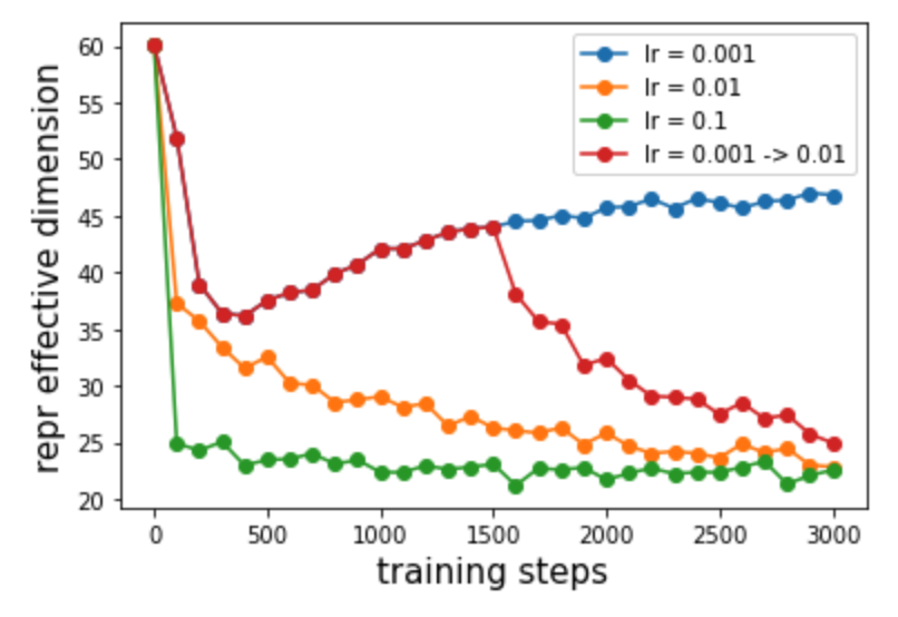
Since a 1D embedding is already sufficient, an extreme case with higher-dimensional embeddings is that different embedding dimensions behave identically. In that case, the effective subspace dimension of the embeddings is actually 1. While reality may not be so extreme, this motivates us to measure the effective dimensionality of representations, which may be related to representation collapse observed in LLMs.

For an embedding matrix, we perform principal component analysis (PCA), treat the explained variance ratios as a probability distribution, compute its entropy \(S\), and define the effective dimension as \(n_{\rm eff} = \exp(S).\)

Taking \(V = 100\) and \(D = 100\), we indeed observe representation collapse, which becomes more pronounced for larger learning rates.

Loss scaling laws

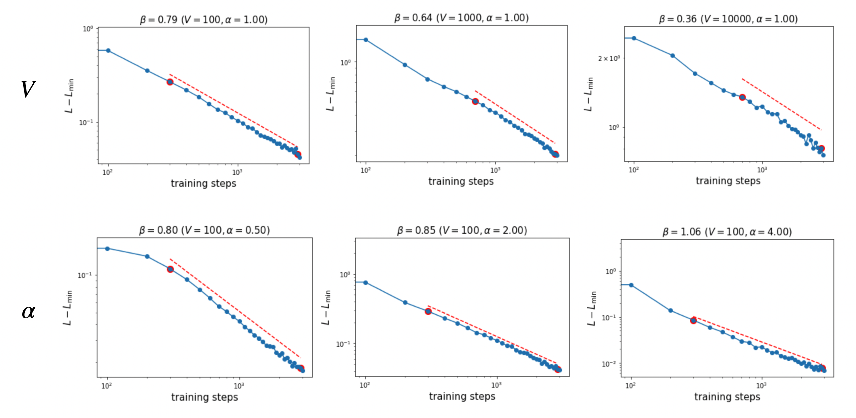
We study temporal scaling of the form \(L - L_{\rm min} \propto t^{-\beta},\) where \(\beta\) measures the speed of loss decay. We vary \(\alpha\) and \(V\) and examine how \(\beta\) depends on them. We fix \(D = 100\) and learning rate \(\text{lr} = 0.001\).

We find that:

• larger \(V\) leads to smaller \(\beta\);
• larger \(\alpha\) leads to larger \(\beta\).

Both trends are intuitive: larger \(V\) or smaller \(\alpha\) corresponds to a harder task.

Learning rate decay

We next ask whether late-stage learning rate decay is helpful in this toy setup. We find that learning rate decay indeed helps, and the improvement becomes larger as the system size increases (i.e., larger embedding dimension \(D\)). We train for 2000 steps with \(\text{lr} = 0.01\), then linearly decay the learning rate from 0.01 to 0.001 over the final 1000 steps. We fix \(V = 100\) and \(\alpha = 1\).

How can we understand this? When the system has many degrees of freedom, and each update is normalized, many degrees of freedom may update in similar directions. Their combined effect can be too large, causing overshoot. In this case, reducing the learning rate is necessary to avoid overshooting.

Learning rate warmup

Can our experiments shed light on the necessity of learning rate warmup? In the representation collapse section, we showed that large learning rates lead to more severe representation collapse—this is one possible explanation.

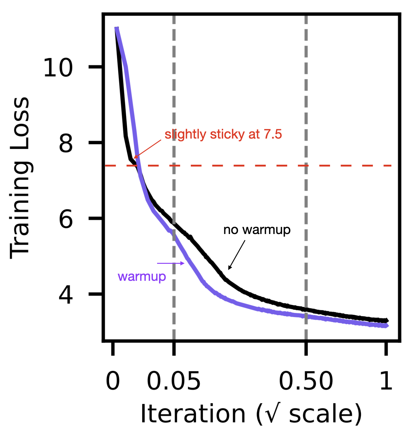
Here we provide another observation. In Analyzing & Reducing Learning Rate Warmup (paper), the authors found that without warmup, training descends faster initially but becomes slightly sticky around loss ≈ 7.5, after which it becomes slower than training with warmup:

How should we interpret this value 7.5? Using our Unigram model, if we take \(V = 50304\) (NanoGPT) and \(\alpha = 1\) (Zipfian), we can compute the entropy to be 7.57. This may not be a coincidence.

With a relatively large initial learning rate, the model may overly exploit Unigram token frequencies to reduce loss quickly, but because the steps are too large, it fails to capture more subtle structures in the data (Bigram, Trigram, or longer-range correlations). As a result, the model is attracted to a Unigram “saddle-point solution,” and escaping from it requires more time. Of course, this is only a hypothesis, and more complex toy models are needed to test it.

Finally, from the perspective of neuron activations, there is another possible explanation: excessively large early learning rates may cause neurons to die more quickly. We discussed this possibility in a previous blog post.

Code

Google Colab notebook available here.

Citation

If you find this article useful, please cite it as:

BibTeX:

@article{liu2026fine-unigram-toy-1,
  title={Unigram toy model is surprisingly rich -- representation collapse, scaling laws, learning rate schedule},
  author={Liu, Ziming},
  year={2026},
  month={January},
  url={https://KindXiaoming.github.io/blog/2026/unigram-toy-1/}
}