Sparse attention 4 -- previous token head

Author: Ziming Liu (刘子鸣)

Motivation

In sparse-attention-2, we found that a single-layer attention model without positional embeddings cannot reliably copy any earlier token based on position. In this article, we demonstrate how positional embeddings enable the model to learn a previous-token head.

Problem setup

Dataset
The task is to copy the previous token. Taking context length = 4 as an example, this corresponds to
\([A][B][C][D] \rightarrow [C]\).

Model
We stick to the toy model from the previous blog, with the addition of a positional embedding layer. The model consists only of a Token Embedding layer, a Positional Embedding layer, an Unembedding layer, and a single Attention layer, with no MLP layers.

With positional embeddings, the previous-token head can be easily learned

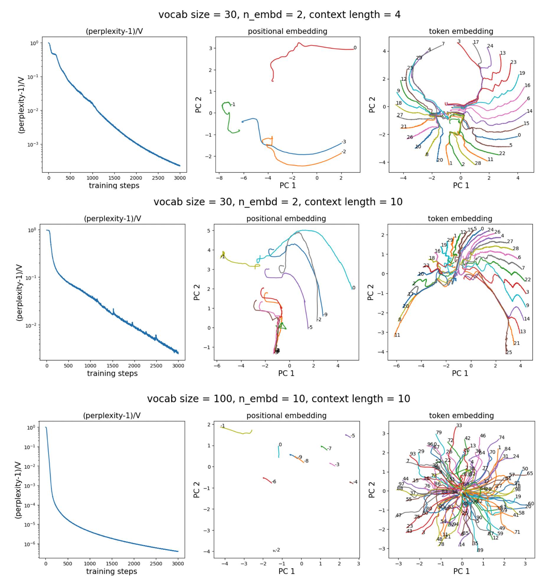
We choose context length 4, vocab size 30, and embedding dimension 2. The left plot shows that the task cannot be learned without positional embeddings. The middle plot shows that the task can be reasonably learned with positional embeddings. The right plot shows the evolution of the positional embeddings: the positional embedding of the previous token (-1) moves in the opposite direction from tokens at other positions (0, -2, -3). The separation direction is roughly \(s = (1,1)^T\). When projecting positional embeddings along \(s\), \(p_{-1}\) is negative, while \(p_0, p_{-2}, p_{-3}\) are positive.

What’s happening?

We can compute the \(W_QW_K^T\) matrix, obtaining

Note that \(s^T W_QW_K^T s = -1.1 < 0\). If two positional embeddings have the same (opposite) sign along \(s\), they will receive less (more) attention. As a result, since only \(p_{-1}\) has the opposite sign relative to \(p_0\), the attention is biased toward the previous token.

Hyperparameter dependence

However, the task is not solved exactly, but only approximately. With larger vocab size or larger context length, the task becomes harder for the model to approximate, so the relative perplexity \(({\rm perplexity} - 1)/V\) increases. In contrast, a larger embedding dimension helps reduce the relative perplexity.

I want to argue that the need for higher embedding dimensions suggests inefficiency. Ideally, a 1D positional embedding should suffice if the attention kernel is chosen appropriately (here the attention kernel is the inner product).

Dependence on learning rate

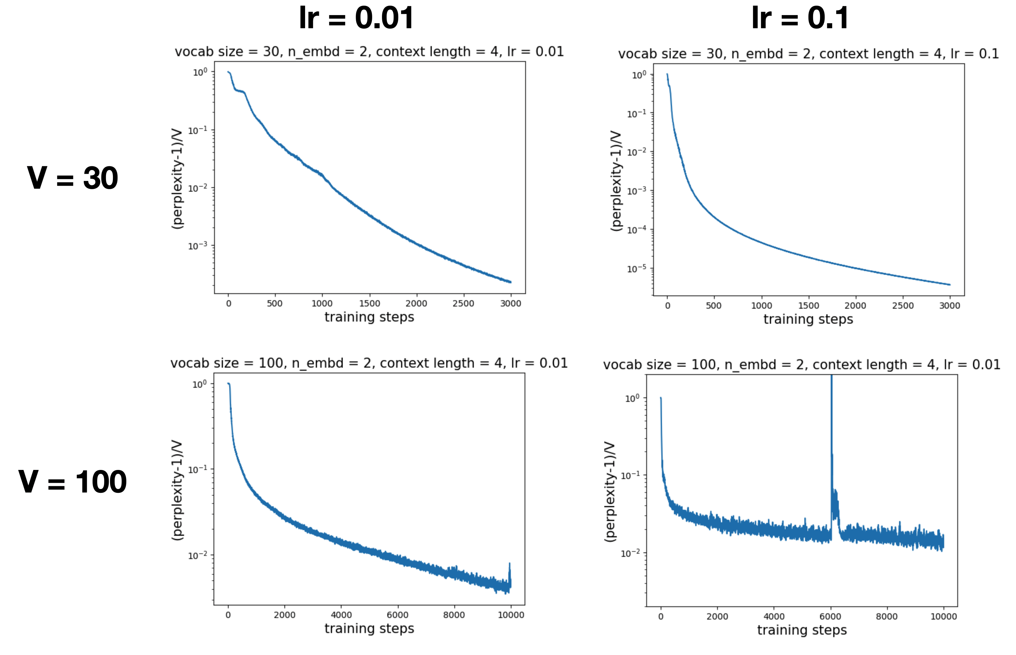
When \(V = 30\), a learning rate of 0.1 is faster than 0.01. However, when \(V = 100\), a learning rate of 0.1 leads to slower learning than 0.01.

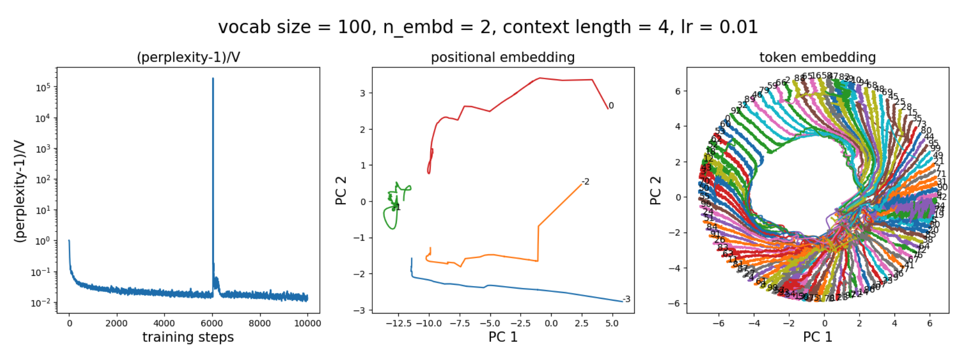
It appears that lr = 0.1 still learns the previous-token head (since there exists a separation direction in the positional embeddings):

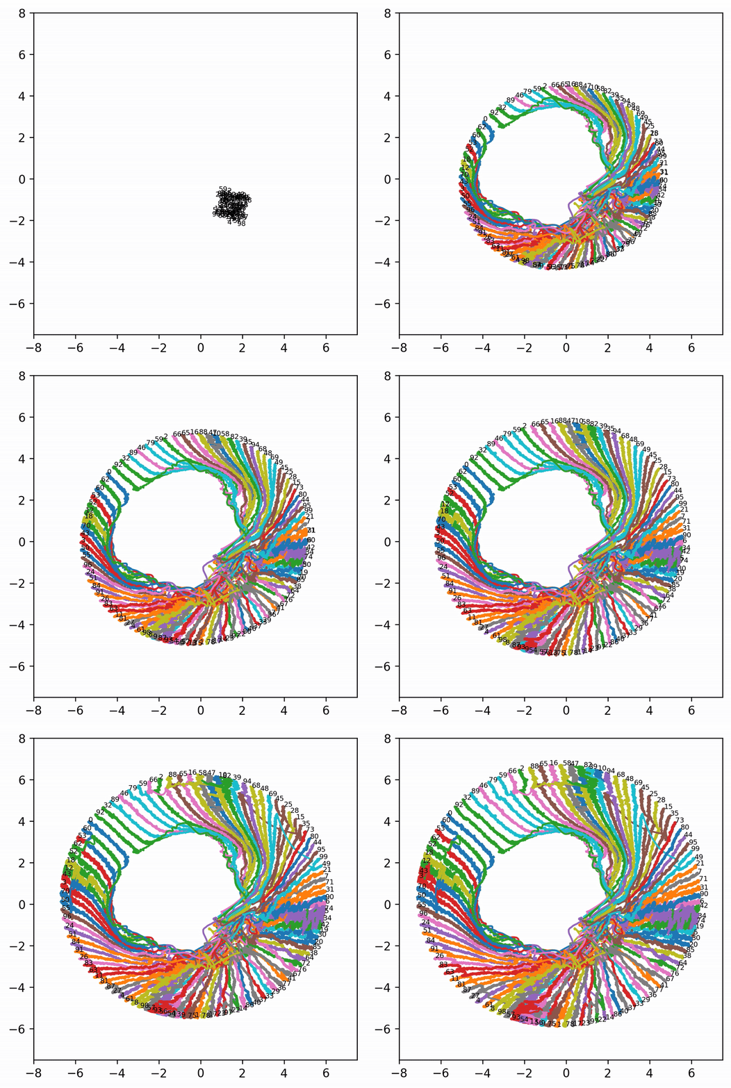
However, because the learning rate is too large, the token embeddings fluctuate wildly and fail to converge to a maximally separable solution (nearby points are placed equidistantly on a circle). The learning rate is so large that tokens swap positions. The loss spike around 6000 steps corresponds to this swapping process, during which the model is confidently wrong for some tokens, leading to very large losses. This GIF illustrates the behavior more clearly:

Note that the tokens in this task have no semantic meaning. The reason they form a circle is simply maximal distinguishability, and their ordering is random. The loss spike corresponds to jumping from one order to another order.

Learning rate decay

The observation above suggests a possible reason for why learning rate decay is needed. When two token embeddings are very close to each other, the learning rate should be small enough so that (i) swampping cannot happen (be trapped in one basin of attraction), otherwise creating loss spikes and (ii) can converge smoothly to the bottom of the basin of attraction (maximal separation of token embeddings). In this article, all tokens have the same frequency so they form a circle due to symmetry. But for natural languages, tokens have different frequencies and so different token embeddings may have different norms, requiring different learning rates. How we can adjust learning rates based on token frequency (which can be easily known) is investigated in future posts.

Generality

• Although we exemplify the analysis with the previous token (the token right before the current token), the analysis applies to any earlier token at any position, e.g., 3 tokens away in the past.

Code

Google Colab notebook available here.

Citation

If you find this article useful, please cite it as:

BibTeX:

@article{liu2026sparse-attention-4,
  title={Sparse attention 4 -- previous token head},
  author={Liu, Ziming},
  year={2026},
  month={January},
  url={https://KindXiaoming.github.io/blog/2026/sparse-attention-4/}
}