Optimization 4 -- Loss Spikes

Author: Ziming Liu (刘子鸣)

Motivation

During neural network training, we often observe sudden loss spikes. The goal of this article is to construct a minimal model that helps us understand the origin of such loss spikes.

2D toy model

We aim to regress the function \(y(x) = x^2\) using an MLP. I first found that a 2-layer MLP is sufficient to produce loss spikes. Then I found that a width of 2 is already enough. Further, removing biases does not eliminate the spikes. At this point, the model has only four parameters, and clear symmetries emerge: the two weights in the first layer are almost identical up to a sign flip, and the two weights in the second layer are nearly the same.

After all these simplifications, we are naturally led to study the following toy model, which has only two parameters \((a, w)\): \(f(x) = a \bigl(\sigma(wx) + \sigma(-wx)\bigr),\ \sigma(x) = {\rm silu}(x) = \frac{x}{1+e^{-x}}\)

We train this “model” to fit the squared function for \(x \in [-1, 1]\).

Loss spikes

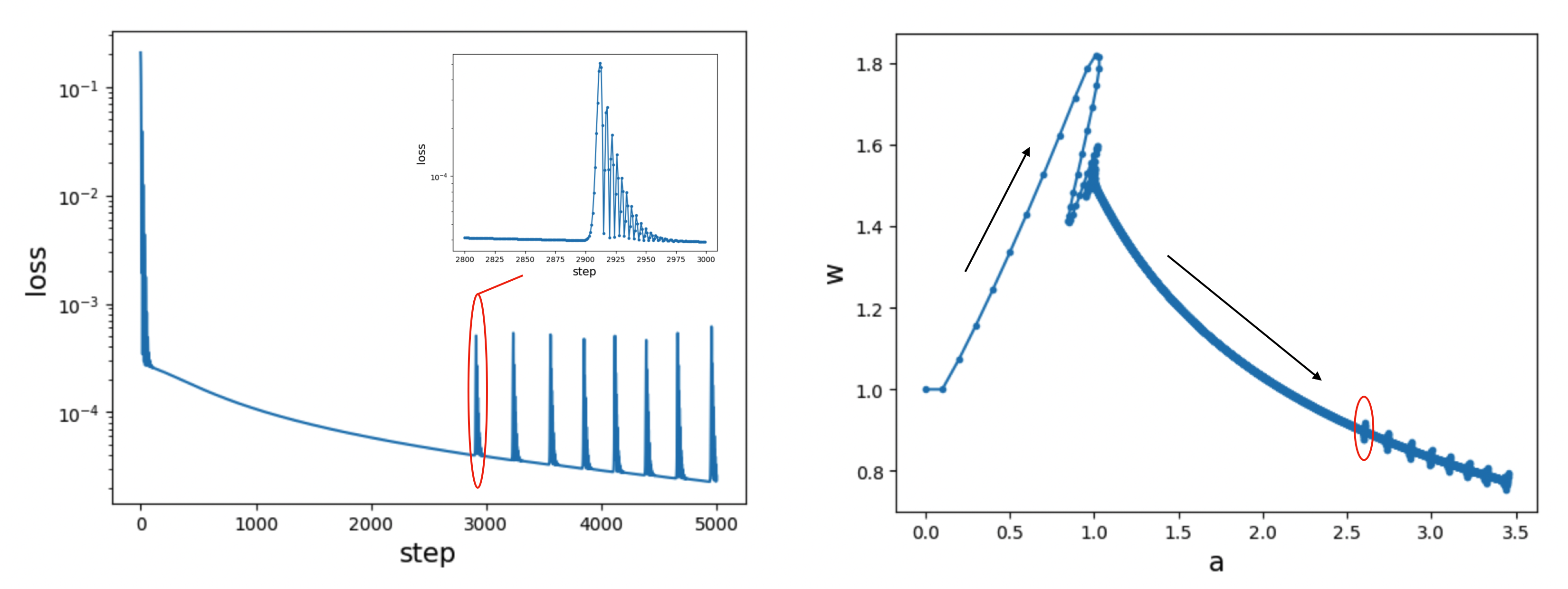
We initialize \(w = 1\) and \(a = 0\), and train using the Adam optimizer (learning rate 0.1) for 5000 steps. The left plot shows that the training loss exhibits spikes. When zoomed in, each spike is asymmetric: a rapid instability followed by a gradual recovery. The right plot shows the training trajectory, which appears to consist of two phases whose dominant movement directions are nearly orthogonal. Loss spikes occur in the second phase, where the parameters seem to navigate a long, narrow valley—known as a river-valley landscape.

Loss landscape

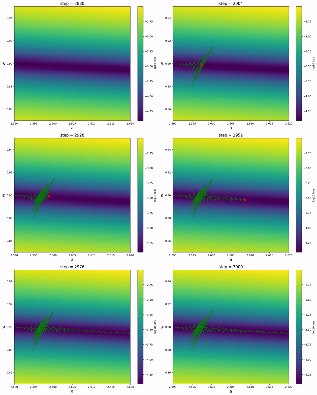
We further verify the presence of a river-valley landscape:

Loss spikes occur when the effective learning rate becomes too large relative to the edge-of-stability threshold \(2/C\), where \(C\) denotes the curvature (see, e.g., edge of stability and the slingshot mechanism). We measure that the curvature at the bottom of the valley is approximately proportional to \(a\) (see the left plot below). As \(a\) increases, \(C\) increases, making spikes more likely.

Periodicity

After the first spike, subsequent spikes appear periodically, roughly every 250 steps. As discussed above, the occurrence of a spike depends on two factors: the effective learning rate and the curvature. For Adam, the effective learning rate depends on the second-moment accumulator, exp_avg_sq, which is shown in the middle plot below. Aside from the initial growth and the spikes themselves, exp_avg_sq decays exponentially as \(0.999^t\), where \(0.999\) is Adam’s \(\beta_2\).

A plausible explanation for the spike periodicity is therefore the following: each spike amplifies exp_avg_sq by some constant factor, and the interval between spikes corresponds to the time it takes for this factor to decay back to 1 (or slightly above 1, since the curvature increases slowly over time). The curvature is roughly a linear function of \(a\) (left plot), and Adam statistics are also shown in the right plot.

If this explanation is correct, we would expect a larger \(\beta_2\) to result in less frequent spikes, which is indeed what we observe.

Video

A close-up view of how a spike unfolds:

It’s interesting to observe that the parameter could temporarily go backwards along the river during the spike, probably due to the entropic force.

Code

Google Colab notebook available here.

Citation

If you find this article useful, please cite it as:

BibTeX:

@article{liu2026optimization-4,
  title={Optimization 4 -- Loss Spikes},
  author={Liu, Ziming},
  year={2026},
  month={January},
  url={https://KindXiaoming.github.io/blog/2026/optimization-4/}
}