Optimization 2 -- Elementwise Scale Reparametrization

Author: Ziming Liu (刘子鸣)

Motivation

In the previous blog, we showed that a re-parametrization trick can significantly speed up optimization. The key ideas were: (1) decompose the weight as \(W = s \hat{W}\), where \(s\) is a scale factor and \(\hat{W}\) has unit norm and represents the direction; (2) make both \(s\) and \(\hat{W}\) learnable. After each update, we rescale \(\hat{W}\) back to the unit sphere and adjust \(s\) accordingly so that the product \(W = s \hat{W}\) remains unchanged.

In this blog, we continue along this direction, but with two additional questions in mind:

• The toy example in the previous blog is too simple. We would like to extend it to a slightly more realistic setup (a linear layer).
• Previously, we used a scalar \(s\) to normalize the vector. Is it possible to perform the normalization element-wise instead?

Failure mode when normalizing element-wise

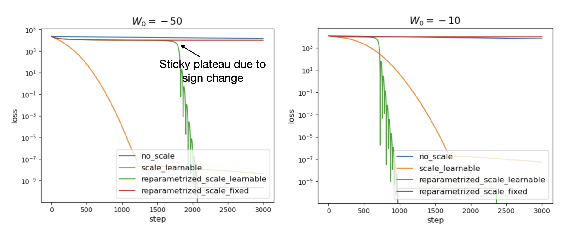
In the previous blog, the toy example was two-dimensional. This was a deliberate choice, because the one-dimensional case has a failure mode: when \(s\) is not learnable, the weight cannot change sign, since \(\hat{W}\) can only take values \(+1\) or \(-1\), which are not connected. This issue does not arise in dimensions greater than or equal to two, because unit vectors form a continuous manifold and the two poles are connected, hence reachable through learning.

In practice, however, we find that as long as \(s\) is learnable, the weight parameter can change its sign even in 1D, because \(s\) itself can change sign (by crossing zero) during training.

We numerically test the four modes discussed in the previous blog for the 1D case, with initial weight \(W_0 = -1\) and target \(W^* = 100\). With re-parametrization and a learnable scale, learning is much faster than in the other modes.

Linear regression

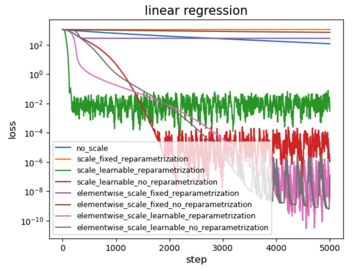
We consider a linear regression setup where \(y = W^* x\), with \(x \in \mathbb{R}^{10}\), \(y \in \mathbb{R}^{10}\), and \(W \in \mathbb{R}^{10 \times 10}\) (for simplicity, we ignore the bias term). We draw \(x \in \mathbb{R}^{10}\) from a standard Gaussian distribution. To generate labels \(y\), we deliberately make \(W^*\) anisotropic by setting \(W^*_{ij} = s_i s_j v_{ij},\) where \(v_{ij}\) is drawn from a standard Gaussian, and \(s_i = 10^{-1 + 2 i / 9}, \quad (i = 0, 1, \dots, 9),\) which spans a wide range in \([0.1, 10]\). The loss function is the MSE loss, and we use the Adam optimizer with learning rate \(\eta = 0.01\).

We compare the following eight modes:

• 8 = [Scalar, Matrix (element-wise)] × [fixed, learnable] × [Re-parametrization, No re-parametrization]

Observations:

• Scalar normalization is faster than element-wise normalization in the early stage (compare green and pink).
• Re-parametrization helps during early training, but not as much—and can even slow things down—during later training (e.g., compare green and red; compare pink and gray).
• A learnable scale is essential for element-wise normalization (compare purple and pink; compare brown and gray).

Code

Google Colab notebook available here.

Citation

If you find this article useful, please cite it as:

BibTeX:

@article{liu2026sparse-optimization-2,
  title={Optimization 2 -- Elementwise scale reparametrization},
  author={Liu, Ziming},
  year={2026},
  month={January},
  url={https://KindXiaoming.github.io/blog/2026/optimization-2/}
}