Physics of Feature Learning 1 – A Perspective from Nonlinearity

Author: Ziming Liu (刘子鸣)，Zhiyun Zheng (郑植匀)，Qingyu Qu（屈清宇）

Motivation

Please Read our latest post Physics of AI Requires Mindset Shifts for general philosophy.

While reading Yuandong Tian’s work on explaining grokking through feature learning, I found the proposed three-stage dynamics of feature learning particularly intriguing. However, grokking itself has some special characteristics (e.g., the modular addition dataset), which led me to wonder whether feature learning could be studied in a more standard setting. This motivated the low-dimensional regression example explored below.

Rather than starting from mathematical derivations, I decided to go straight to experiments. Beyond plotting the loss, we also wanted to define observables that characterize features. One of the most basic observables is the number of nonlinear neurons. This measure does not care about the specific form of the features, only whether they are nonlinear.

To define neuron activation cleanly, we use ReLU activations. A neuron is considered nonlinear if it is activated for some inputs and inactive for others.

Problem Setup

We consider the following regression function:

We use an MLP with 10-dimensional input, 100 neurons in the first hidden layer, 100 neurons in the second hidden layer, and a single output. We denote the architecture as ([10, 100, 100, 1]). Inputs are sampled from a standard Gaussian distribution, with a total of 500 samples. The training objective is MSE loss, optimized using Adam (learning rate \(10^{-3}\), full batch).

Observation: Four Phases During Training

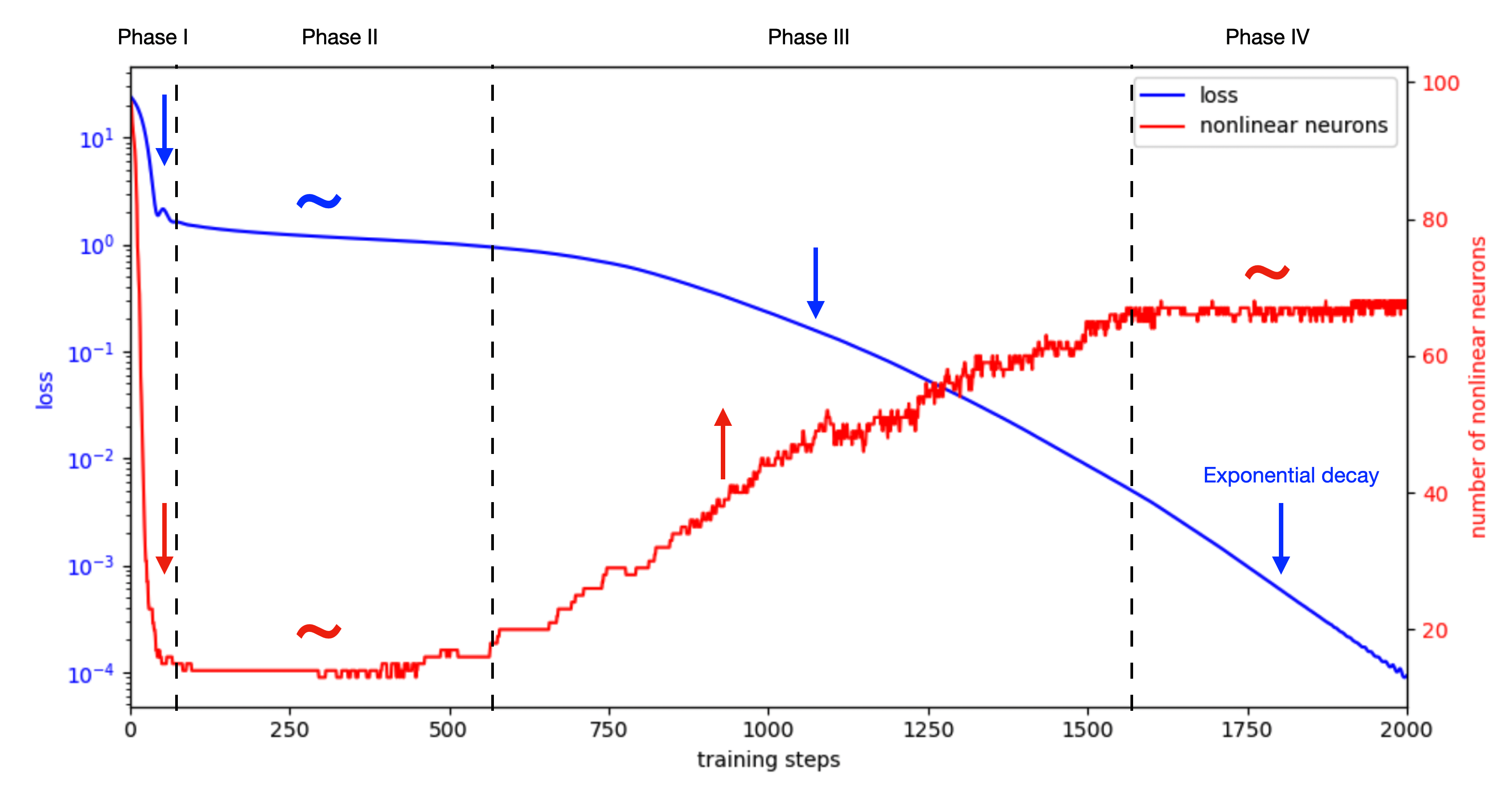
We find that all 100 neurons in the first hidden layer remain nonlinear throughout training. In contrast, the number of nonlinear neurons in the second hidden layer exhibits non-trivial dynamics. Therefore, all plots below focus on the evolution of nonlinear neurons in the second hidden layer.

Empirically, the training dynamics appear to consist of four phases:

• Phase I (first ~50 steps)
  The loss decreases rapidly, while the number of active neurons drops sharply.
  Hypothesis: the model is removing irrelevant features.

• Phase II (50–500 steps)
  The loss plateaus around 1, and the number of active neurons remains roughly constant (around 14).
  Hypothesis: the model is stuck near a saddle point, leading to slow learning.

• Phase III (500–1500 steps)
  The loss decreases slowly, while the number of active neurons increases.
  Hypothesis: this corresponds to genuine feature learning.

• Phase IV (after ~1500 steps)
  The loss decreases rapidly (exponential convergence), while the number of active neurons stays constant.
  Hypothesis: the model is fine-tuning features, or fine-tuning the final linear layer.

There are many interesting questions one could study here.

Curiosity-Driven Questions

• Why does Phase I remove so many features?
  Speculation: is this related to optimization tricks in LLMs? For example, do weight decay and learning-rate warmup mainly serve to prevent excessive feature removal in this phase?

• Phase II appears “sticky.” How should we better understand the meaning of this solution?
  Speculation: is the loss plateau simply the result of linear regression?

• How do nonlinear features emerge in Phase III?

• What determines the exponential convergence rate in Phase IV?
  Speculation: once features are learned, does the problem effectively reduce to linear regression, which we know converges exponentially?

A Linear Regression Perspective

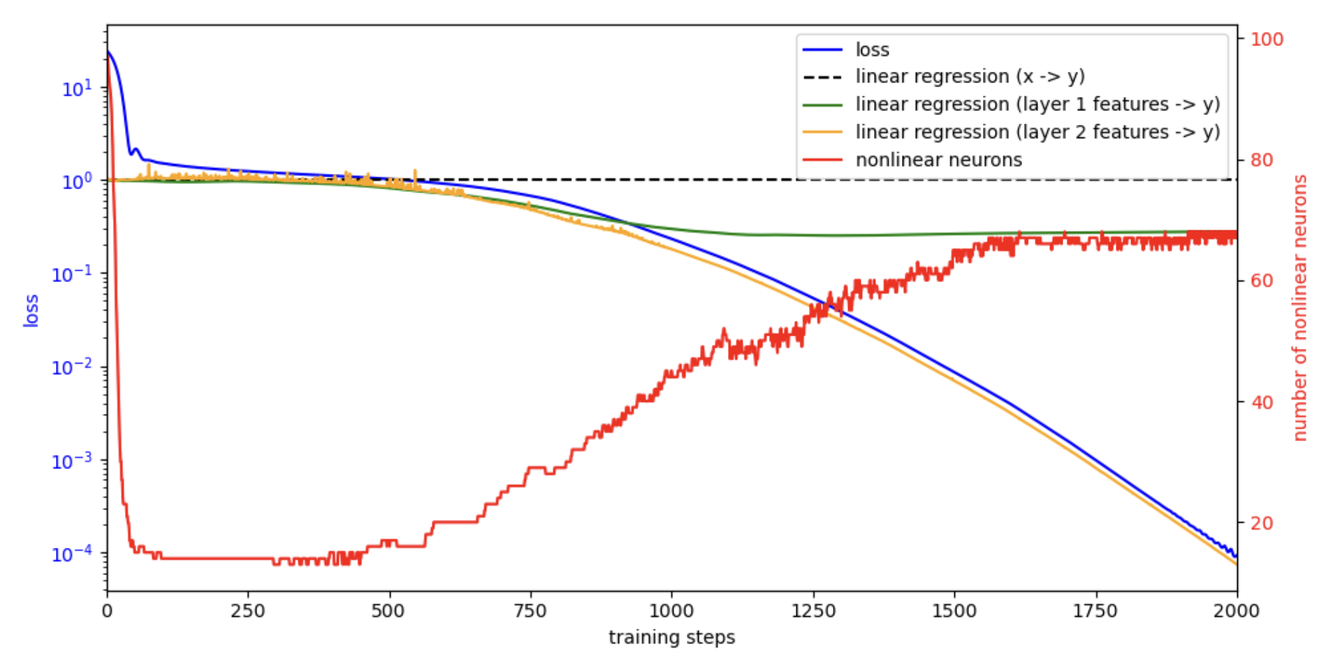
To better understand the dynamics, we analyze the model from a linear regression viewpoint. We compute three linear regression baselines:

where \(f_1\) and \(f_2\) denote the features from the first and second hidden layers, respectively, which evolve during training.

We observe that:

• The loss plateau around 1 corresponds closely to the solution of linear regression.
• In the late stage of training, the blue and orange curves nearly coincide, indicating that the final-layer weights are essentially optimal at every moment, while the features are still being fine-tuned. As a result, the loss continues to decrease.

This is not standard linear regression (where features are fixed and weights evolve), but rather a dual version: features evolve while weights remain near their instantaneous optimum. Interestingly, this still leads to exponential decay. A natural next step is to understand the convergence rate quantitatively.

Code

Google Colab notebook available here.

Observing interesting phenomena and asking good questions is already half the battle. We are still working toward explaining more of these effects. If you have any idea regarding how to understand some of the phenomena, please email me at lzmsldmjxm@gmail.com

Citation

If you find this article useful, please cite it as:

BibTeX:

@article{liu2026feature-learning-1,
  title={Physics of Feature Learning 1 -- A Perspective from Nonlinearity},
  author={Liu, Ziming and Zheng, Zhiyun and Qu, Qingyu},
  year={2026},
  month={January},
  url={https://KindXiaoming.github.io/blog/2026/feature-learning-1/}
}

Text citation:

Liu, Ziming and Zheng, Zhiyun and Qu, Qingyu (January 2026). Physics of Feature Learning 1 – A Perspective from Nonlinearity. KindXiaoming.github.io. https://KindXiaoming.github.io/blog/2026/feature-learning-1/