Diffusion 2 -- Visualizing flow matching, temporal dynamics

Author: Ziming Liu (刘子鸣)

Motivation

I was reproducing Tianhong and Kaiming’s JIT paper, “Back to Basics: Let Denoising Generative Models Denoise”. The first step is to implement the v-prediction baseline on the spiral dataset (Figure 2 in the paper). Reproducing the baseline should be straightforward, but I ended up getting stuck for quite a while. Eventually, I realized that how \(t\) is sampled during training is crucial.

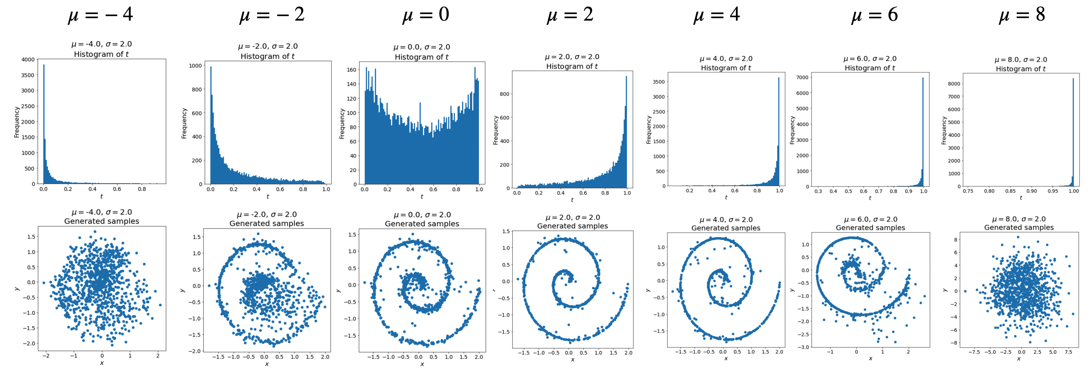
Specifically, \(t\) is sampled from a logit-normal distribution: \(t = \frac{1}{1 + e^{-X}}, \quad X \sim \mathcal{N}(\mu, \sigma^2).\) However, the main paper does not clearly specify how \((\mu, \sigma)\) are chosen. I therefore experimented with different values to understand their effects. Note that \(t = 0\) corresponds to pure noise, while \(t = 1\) corresponds to clean data.

Tweaking \(\mu\) and \(\sigma\)

We first fix \(\sigma = 2\) to ensure sufficient coverage of the time range, and sweep over \(\mu\):

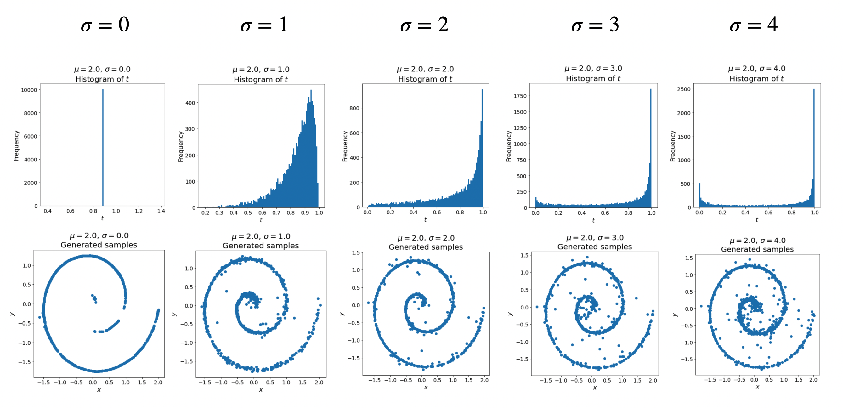
We find that \(\mu = 2\) yields the best generation results. We then fix \(\mu = 2\) and sweep over \(\sigma\):

Somewhat surprisingly, \(\sigma = 0\) can still lead to decent generation quality. We therefore fix \(\sigma = 0\) and vary \(\mu\):

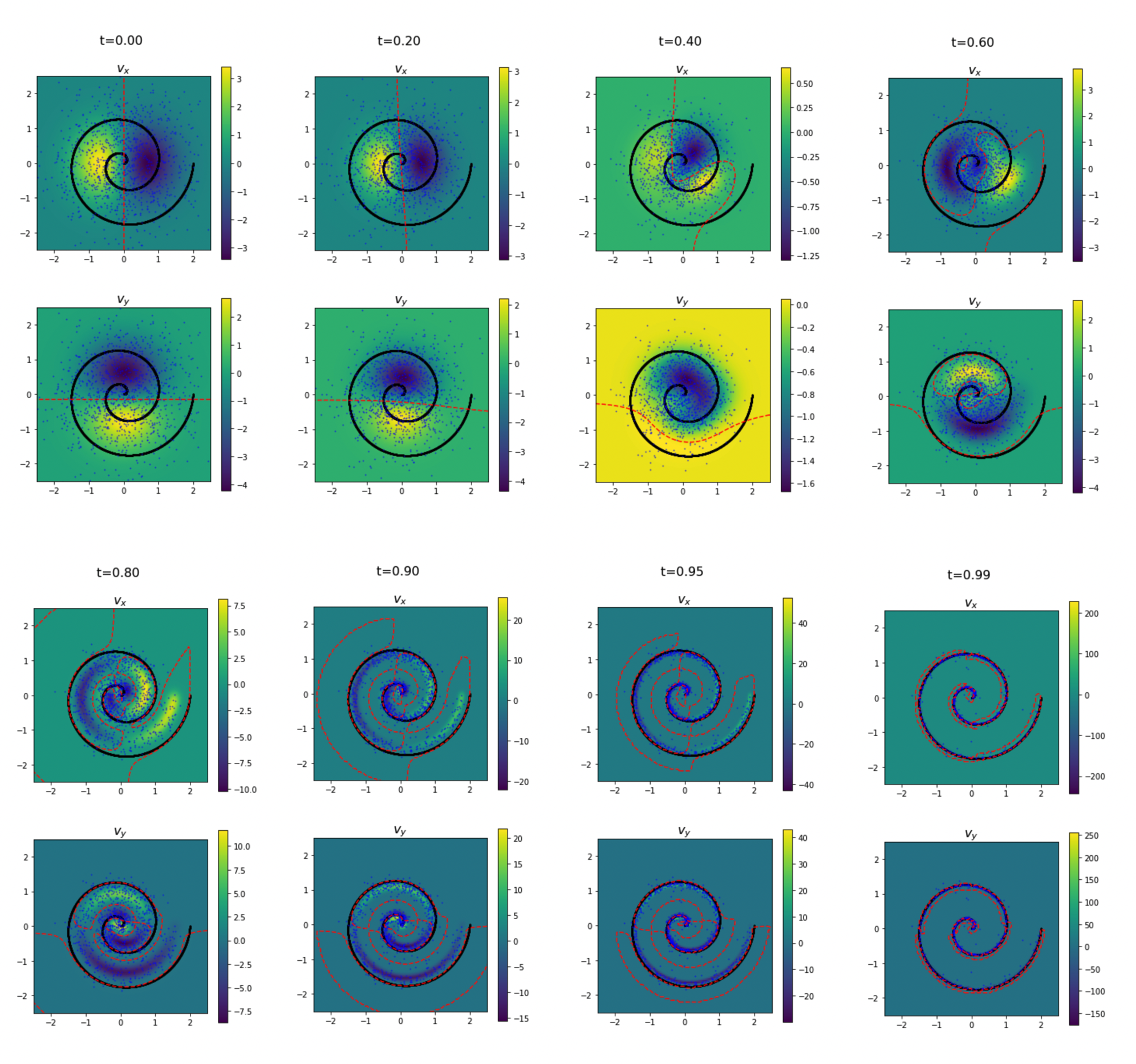
To better understand why \(\sigma = 0\) can still produce good samples, note that \(\sigma = 0\) means training only ever sees a single time \(t = \frac{1}{1 + e^{-\mu}}.\) Below, instead of training a neural network, we numerically estimate the true velocity field and visualize it directly.

Visualizing true velocities

For different values of \(t\), we visualize the velocity field using two color plots (a full vector-field visualization would be difficult to interpret due to potential multi-scale structure). Top: \(v_x\); bottom: \(v_y\). In each subplot, black dots indicate data samples, blue dots indicate generated samples at that time step, and red dashed lines show the zero-level sets.

This makes it clear why training at a single \(t \sim 0.9\) can already yield high-quality samples: the zero-velocity contours align well with the spiral manifold. Under this velocity field, samples naturally converge toward the zero-velocity region.

We also notice that that scale of \(v\) diverges as \(1/(1-t)\) when \(t\to 1\), which is another reason why predicting \(v\) is hard, besides JIT paper’s reasoning about manifolds.

Code

Google Colab notebook available here.

Citation

If you find this article useful, please cite it as:

BibTeX:

@article{liu2026diffusion-2,
  title={Diffusion 2 -- Visualizing flow matching, temporal dynamics},
  author={Liu, Ziming},
  year={2026},
  month={February},
  url={https://KindXiaoming.github.io/blog/2026/diffusion-2/}
}