Depth 4 -- Flat directions (in weight space) are high frequency modes (in function space)

Author: Ziming Liu (刘子鸣)

Motivation

In a recent blog post depth-3, we found that the normalized eigen-spectrum aligns across depths. Although this alignment may not hold in general, it naturally raises an important question: what is the benefit of depth, then?

To address this question, it is not sufficient to only examine eigenvalues—we also need to understand the corresponding eigenvectors. I can think of two ways to visualize eigenvectors:

Load an eigenvector back into a neural network and visualize the resulting network graph.
Study how perturbations along an eigenvector change the network’s output.

In this article, we adopt the second approach. By choosing tasks with 1D input and 1D output, we can visualize each eigenvector as a 1D curve that represents how the learned function changes under a weight perturbation along that eigenvector.

Problem setup

We consider MLPs with hidden width 20, and compare 2-layer and 3-layer architectures. The task is 1D regression, either \(f(x) = x^2 \quad \text{(smooth)}\) or \(f(x) = \sin(5x) \quad \text{(oscillatory)}.\) We sample \(x \sim U[-1, 1]\). The networks are trained using the MSE loss with the Adam optimizer.

After training, we obtain the model parameters \(\theta\). We then compute the Hessian \(H \equiv \frac{\partial^2 \ell}{\partial \theta^2},\) and its eigenvalues \(\lambda_i\) and eigenvectors \(v_i\) satisfying \(H v_i = \lambda_i v_i.\)

The trained network represents a function \(f(x; \theta)\). To understand the functional meaning of an eigenvector \(v_i\), we perturb the parameters along this direction and obtain the perturbed function \(f(x; \theta + a v_i),\) where \(a\) is a small scalar. We visualize the induced functional change as \(\delta f_i \equiv \frac{1}{a}\bigl(f(x; \theta + a v_i) - f(x; \theta)\bigr).\)

Results for \(f(x) = x^2\)

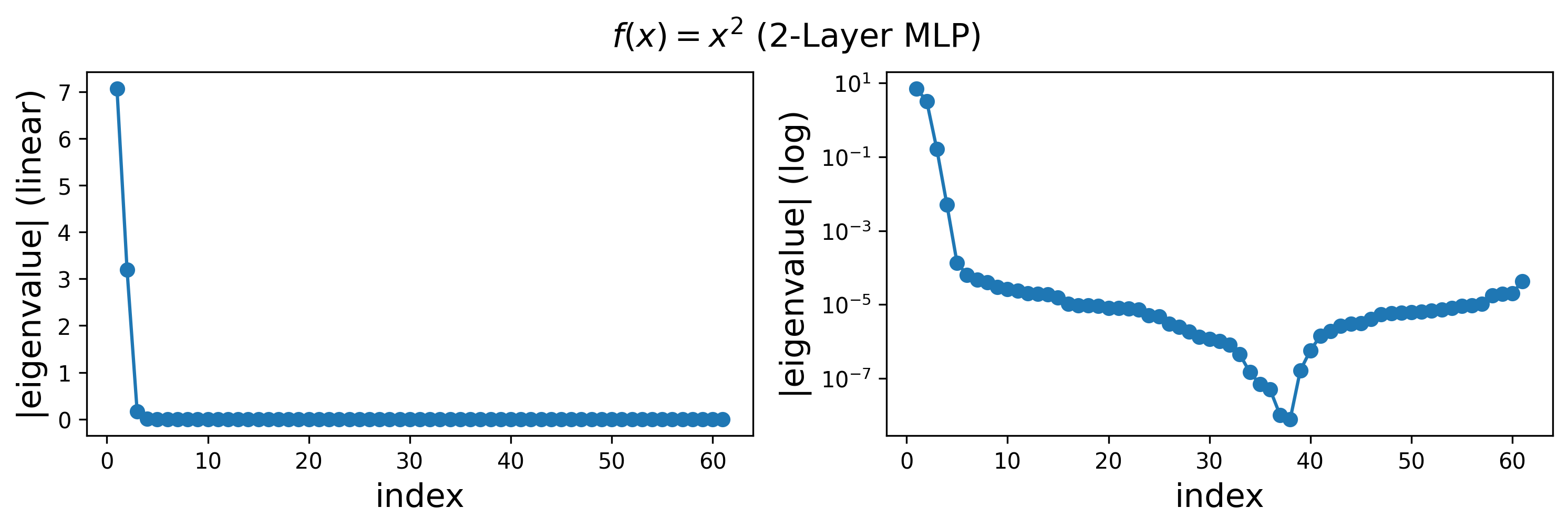
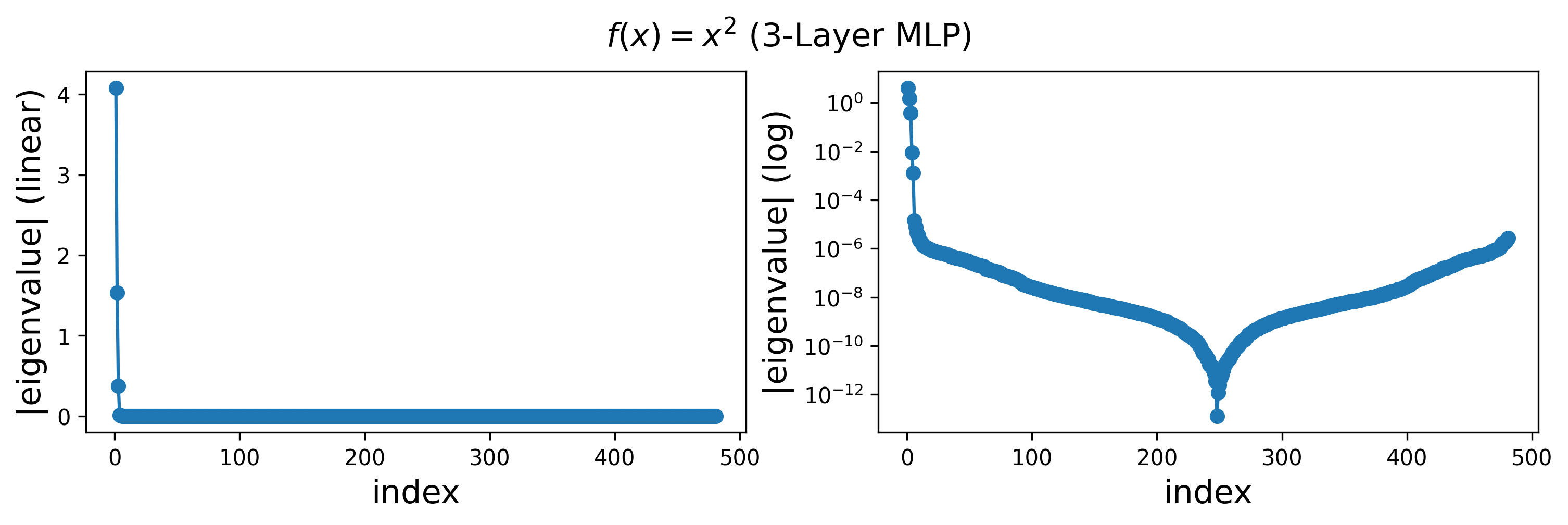
Eigenvalues:

(We take the absoluate value. Note that there are negative eigenvalues at the tail, after the dip)

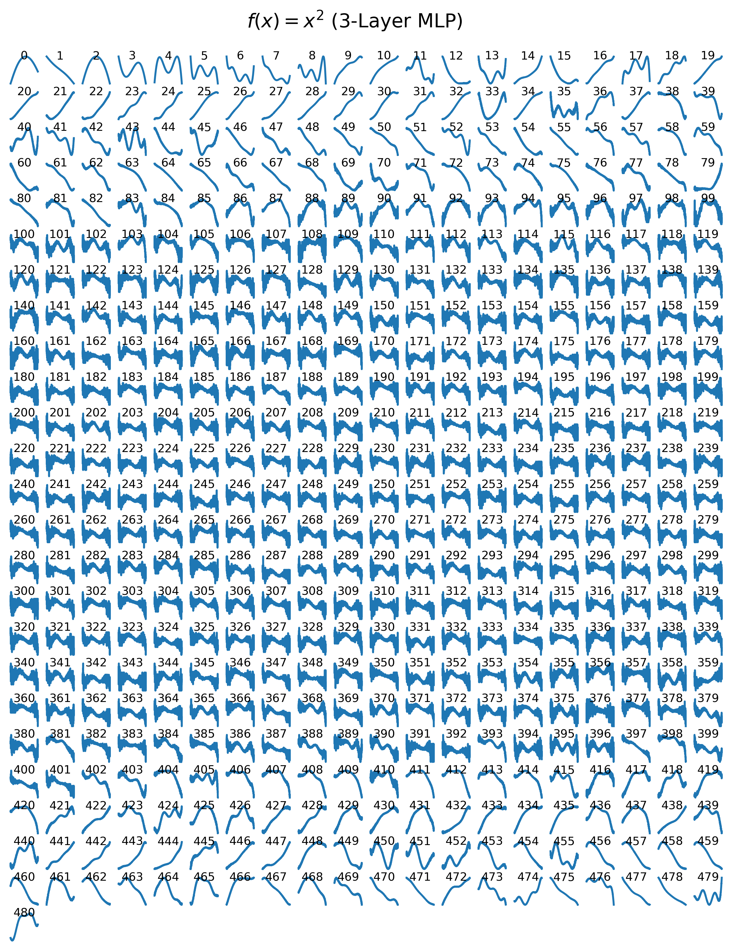
Eigenvectors (perturbed functions):

Results for \(f(x) = \sin(5x)\)

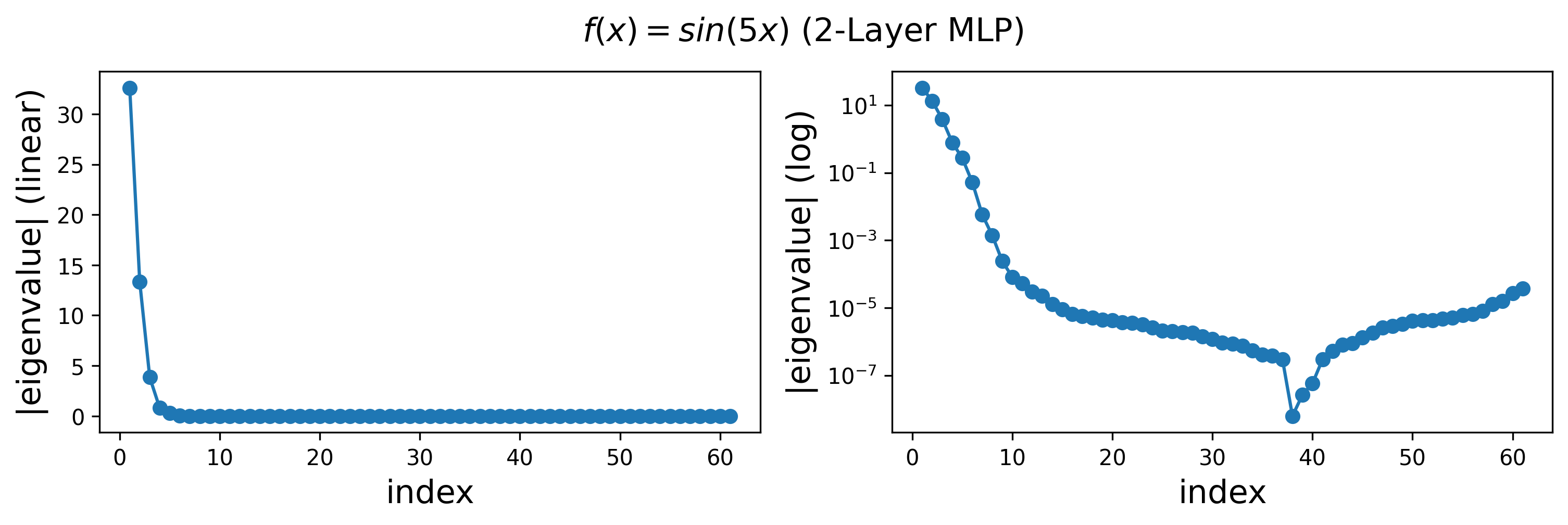
Eigenvalues:

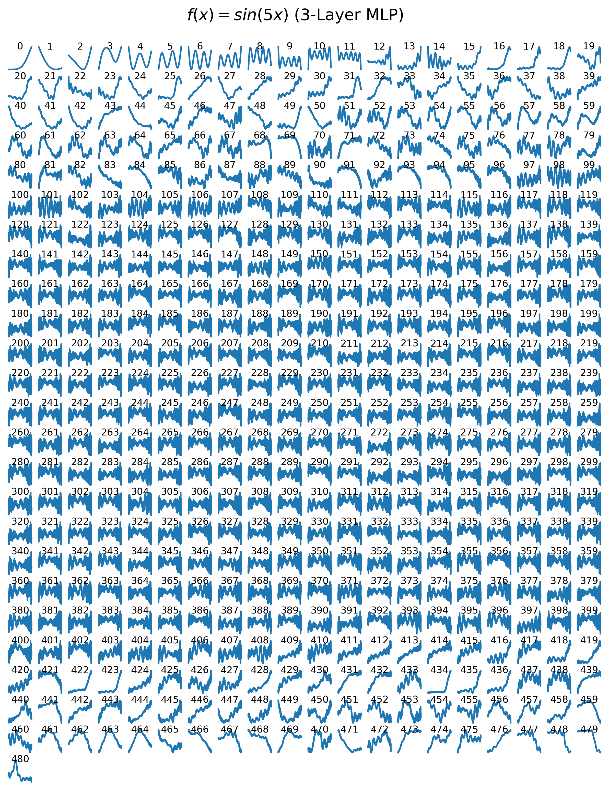
Eigenvectors (perturbed functions):

Comment

In both cases, we find that the leading eigenvalues and eigenmodes are very similar for 2-layer and 3-layer networks. However, the 3-layer networks exhibit more high-frequency modes in the tail of the spectrum. Notably, the highest-frequency modes correspond to eigenvalues that are close to zero.
These results help explain why continual learning is challenging: because these eigenfunctions are not localized, modifying the model to fit a single new data point can induce changes in the function globally, rather than locally.

Code

Google Colab notebook available here.

Citation

If you find this article useful, please cite it as:

BibTeX:

@article{liu2026depth-4,
  title={Depth 4 -- Flat directions (in weight space) are high frequency modes (in function space)},
  author={Liu, Ziming},
  year={2026},
  month={February},
  url={https://KindXiaoming.github.io/blog/2026/depth-4/}
}