Depth 3 -- Fun facts about loss hessian eigenvalues

Author: Ziming Liu (刘子鸣)

Motivation

The loss landscape is a first-principles object governing neural network learning. To characterize the loss landscape, sharpness is commonly used. Specifically, sharpness is defined in terms of the eigenvalues of \(H \equiv \frac{\partial^2 \ell}{\partial \theta^2},\) where \(\ell\) is the loss function, \(\theta\) denotes the model parameters, and \(H\) is the Hessian. Although computing sharpness is prohibitively expensive for large models, it is essential for understanding training dynamics.

In this article, we explore several fun and perhaps surprising facts about sharpness in toy models. While we ultimately hope these observations can shed light on larger models, the goal here is simply to make careful observations and document simple empirical findings.

Problem setup

We use the ResNet toy model described in depth-1. The input (embedding) dimension is \(n_{\rm embd}\). Each block is a two-layer MLP with hidden dimension \(n_{\rm hidden}\). Residual connections are used, and \(n_{\rm block}\) blocks are stacked in depth to form the toy ResNet.

We adopt a teacher–student regression setup: a teacher network generates the targets, and a student network of the same architecture (but with different initialization) is trained using the MSE loss.

Spectrum is gapped, or eigenvalues form clusters

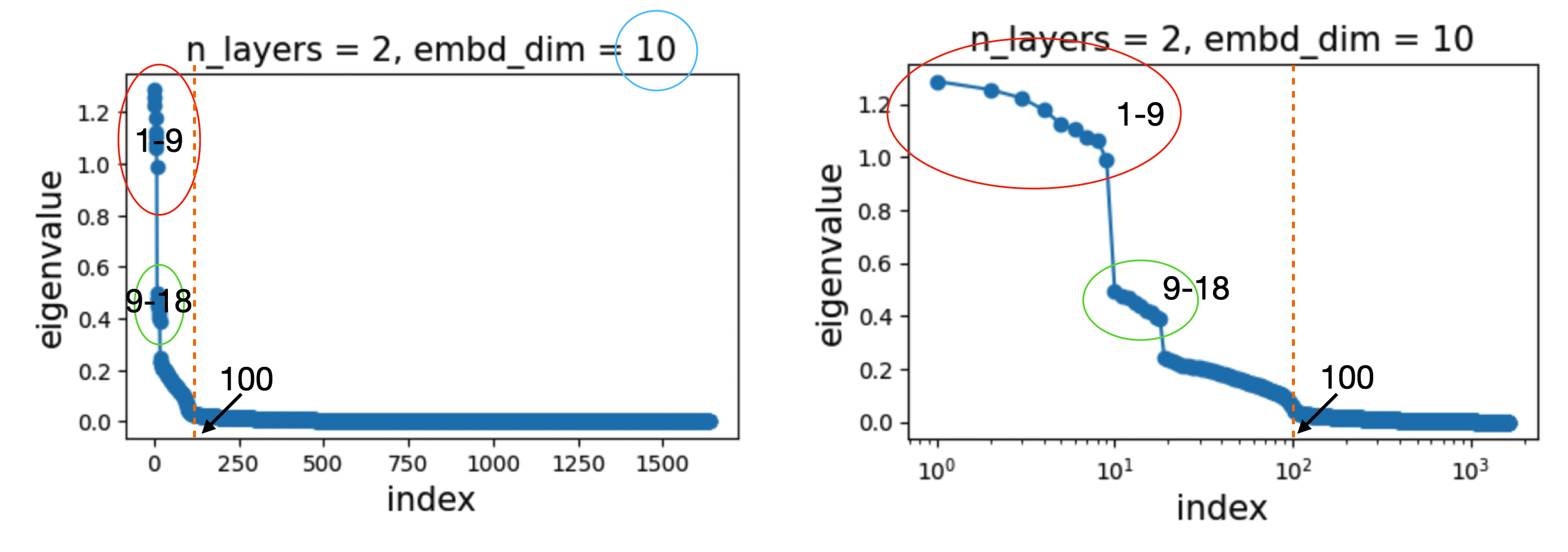
We set \(n_{\rm embd} = 10 \equiv N\), \(n_{\rm hidden} = 40 = 4N\), and \(n_{\rm block} = 2 \equiv D\). The total number of parameters is \(8N^2D = 1600\). Accordingly, the Hessian is a \(1600 \times 1600\) matrix with 1600 eigenvalues. We rank the eigenvalues from largest to smallest:

We find that the spectrum (eigenvalue distribution) is clearly gapped:

The first 9 eigenvalues form a cluster.
The next 9 eigenvalues form another cluster.
The first 100 eigenvalues are significantly larger than zero, while the remaining eigenvalues are close to zero.

These observations naturally raise several interesting questions and hypotheses:

Why 9? We hypothesize that this number is \(N - 1\) (where \(N\) is the embedding dimension). We will show this is true.
Why two large clusters? We initially hypothesize that this is because \(n_{\rm block} = 2\). We will show this is false—there are always two clusters, regardless of how deep the ResNet is.
Why 100? We hypothesize that this number is \(N^2\). We will show this is true.

Experiment 1: Vary \(N\) (embedding dimension)

We vary \(N \in \{10, 15, 20\}\) while keeping \(n_{\rm hidden} = 4N\) and using two blocks.

We observe that:

The number of eigenvalues in each cluster is \(N - 1\).
The number of clusters remains equal to 2.
The number of significantly non-zero eigenvalues is \(N^2\).

Experiment 2: Vary \(D\) (depth)

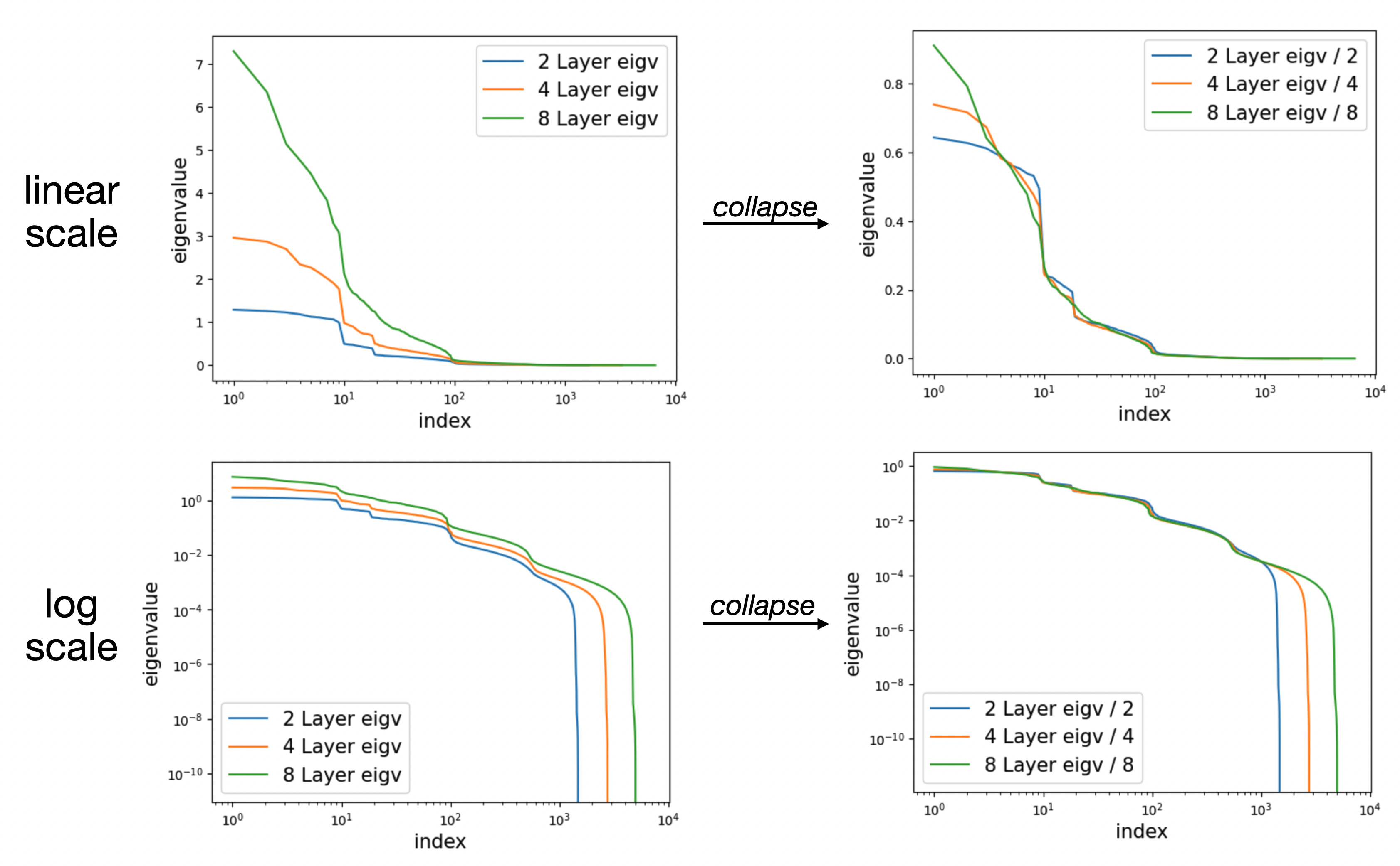
We vary \(D \in \{2, 4, 8\}\) while keeping \(N = 10\) and \(n_{\rm hidden} = 4N\).

We observe that:

The overall eigenvalue structure remains almost unchanged.
The largest eigenvalue (i.e., sharpness) grows roughly linearly with depth.

In fact, if we rescale the eigenvalues by the inverse of the depth, the normalized spectra approximately align across different depths.

Question

Although we made a few conclusions via induction, we did not provide sufficient explanation.
The depth alignment result naturally raises the question: why do we need deep neural networks at all? Given the depth-alignment results, it is very likely that increasing depth mainly introduces more small eigenvalues, whereas increasing width introduces more large eigenvalues. When do large eigenvalues matter, and when do small eigenvalues matter? The eigen-spectrum provides a new perspective into understanding width-depth trade-off.

Code

Google Colab notebook available here.

Citation

If you find this article useful, please cite it as:

BibTeX:

@article{liu2026depth-3,
  title={Depth 3 -- Fun facts about loss hessian eigenvalues},
  author={Liu, Ziming},
  year={2026},
  month={February},
  url={https://KindXiaoming.github.io/blog/2026/depth-3/}
}