Depth 1 -- Understanding Pre-LN and Post-LN

Author: Ziming Liu (刘子鸣)

Motivation

My line of reasoning is as follows.

I want to understand DeepSeek’s mHC paper. To do that, I first need to understand ByteDance’s earlier HC paper.

In the Hyper-connection paper, the introduction states:

The two main variants of residual connections, Pre-Norm and Post-Norm, each make distinct trade-offs between gradient vanishing and representation collapse. Pre-Norm applies normalization operations to the input before each residual block, effectively addressing the problem of gradient vanishing (Bengio et al., 1994; Glorot & Bengio, 2010). However, it can also lead to the issue of collapse in deep representations (Liu et al., 2020), where hidden features in deeper layers become highly similar, diminishing the contribution of additional layers as their number increases. In contrast, Post-Norm applies normalization after the output of each residual block, reducing the influence of a hidden state on subsequent layers. This approach can alleviate the issue of representation collapse but also reintroduces the problem of vanishing gradients. The vanishing gradient and the representation collapse are like two ends of a seesaw, with these two variants making respective trade-offs between these issues. The key issue is that residual connections, including both Pre-Norm and Post-Norm variants, predefine the strength of connections between the output and input within a layer.

In short: Pre-Norm tends to lead to representation collapse, while Post-Norm tends to lead to vanishing gradients. I have heard this conclusion many times, but I never really had the chance to internalize it. The goal of this article is therefore to construct a minimal toy model that helps me better understand these claims about Pre-Norm and Post-Norm.

Problem setup

Dataset
This article focuses only on forward computations, so we do not need to worry about outputs. The inputs are i.i.d. samples drawn from a Gaussian distribution.

Model
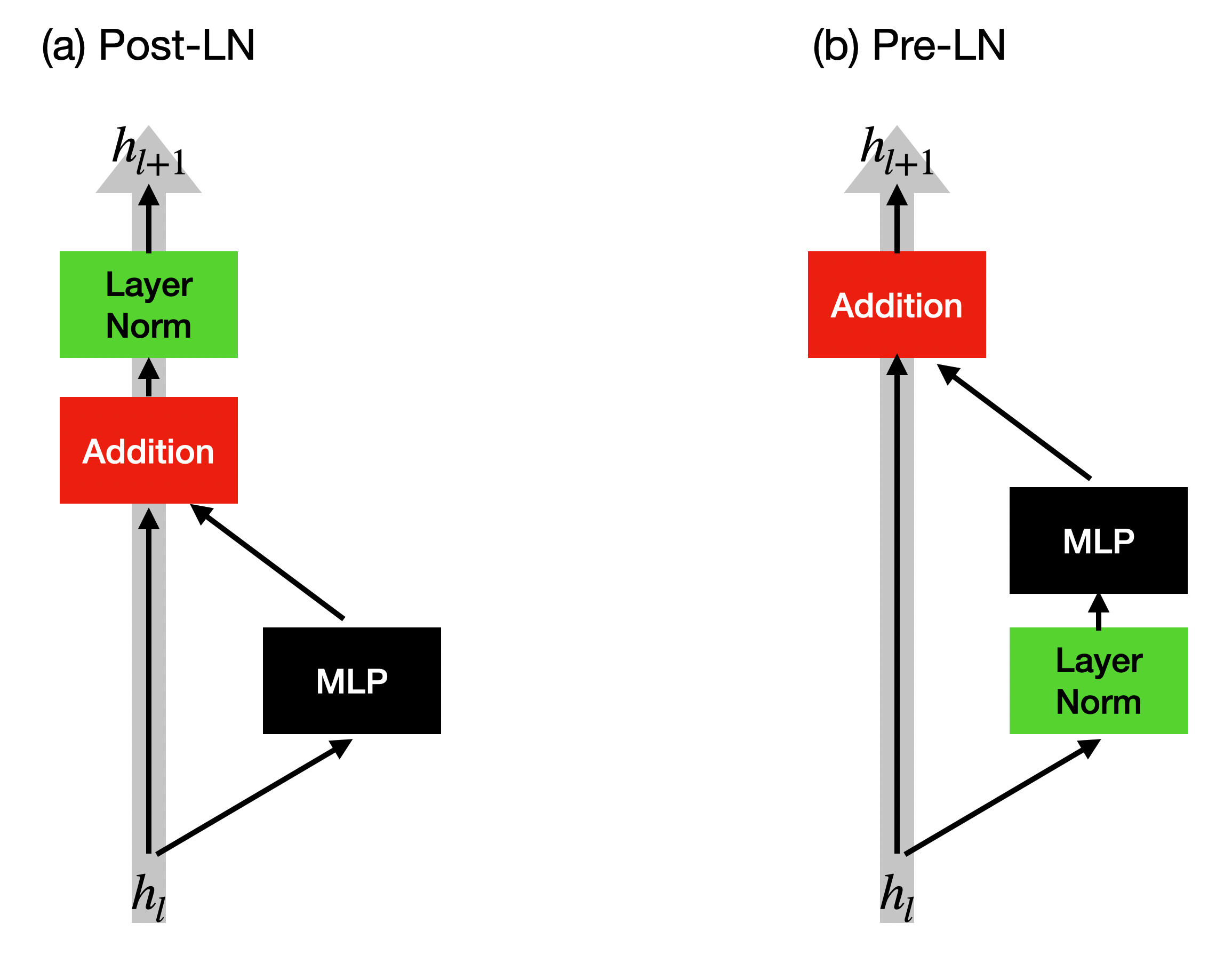
The model consists of residual blocks, where each block is a simple MLP. Each MLP has two fully connected layers, FC1 and FC2. We explicitly control the scale (\(\alpha\)) of FC2 so that we can tune the relative importance of the residual update versus the input.

In practice, during training, \(\alpha\) often increases from 1. Even though we never actually train the model here, we can still vary \(\alpha\) to gain intuition about how a trained model might behave. A large \(\alpha\) means that the update dominates the input, while a small \(\alpha\) means the update is small compared to the input.

The architectures of Post-LN and Pre-LN are shown below.

When the number of samples is much larger than the input dimension, the explained variances from PCA are roughly uniform, so the effective dimension is close to the input dimension. We are interested in how this effective dimension (and other statistics) evolve across layers.

Observation 1: Pre-LN and representation collapse

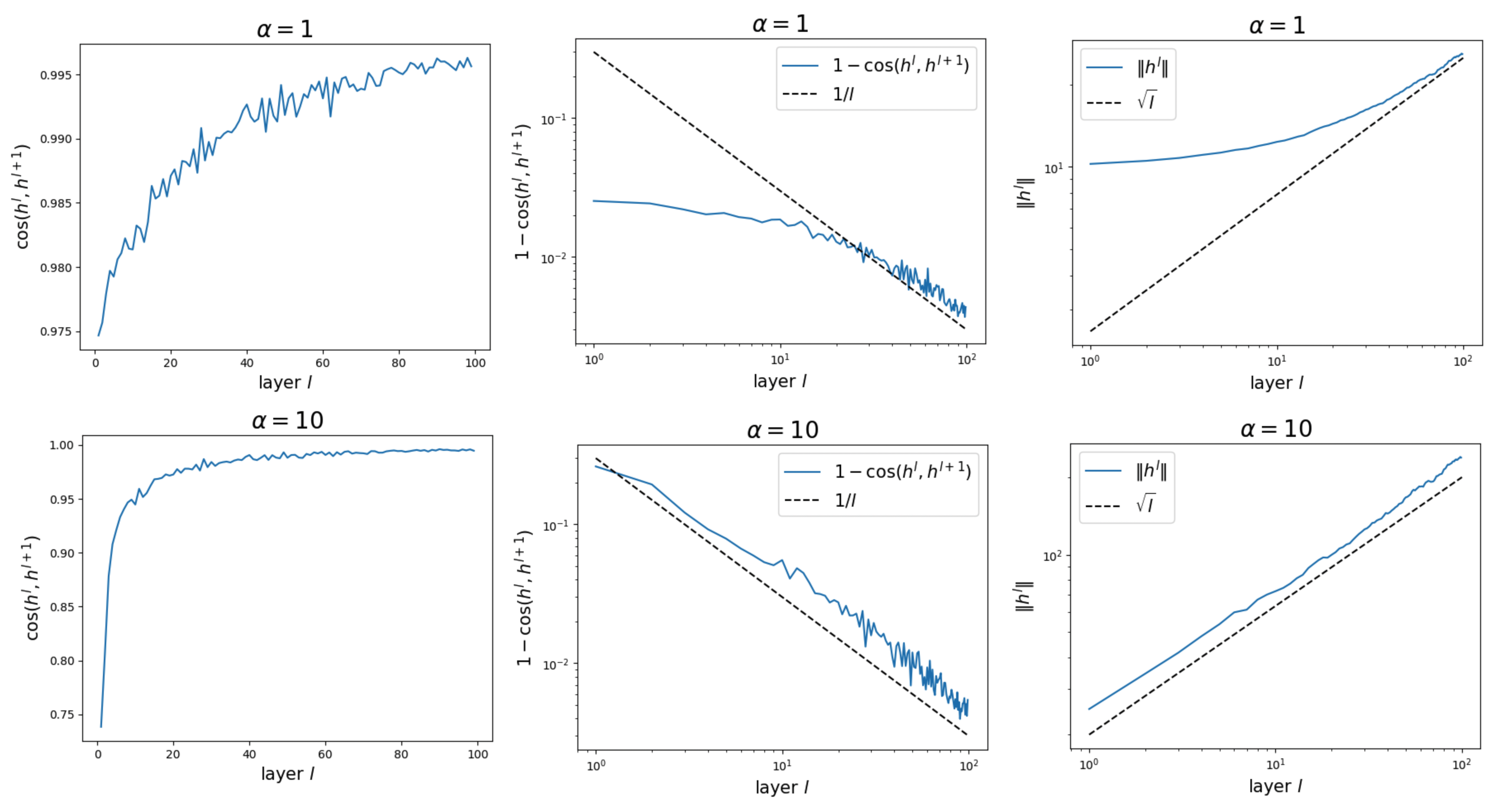
We set the depth to \(L = 100\) layers. Let \(h^l\) denote the residual stream after the \(l\)-th block. We focus on the following quantities:

• the cosine similarity between \(h^l\) and \(h^{l+1}\)
• the norm of \(h^l\)

We observe two asymptotic behaviors:

• \(\lVert h^l \rVert \sim \sqrt{l}\).
  Since the update at each block is random (due to random initialization), the evolution along the depth direction is effectively a random walk. Its variance grows linearly with \(l\), so the norm grows like \(\sqrt{l}\). This likely explains why this paper uses a \(1/\sqrt{L}\) scaling, in order to control the norm.

• \(1 - {\rm cos}(h^l, h^{l+1}) \sim 1/l\).
  The norm of the update is roughly constant, while the norm of \(h^l\) keeps growing. Therefore, the relative angular update satisfies \(\theta \sim 1/\lVert h^l \rVert \sim 1/\sqrt{l}\), which implies \(1 - {\rm cos}(h^l, h^{l+1}) \sim \theta^2 \sim 1/l\).

Observation 2: Post-LN and vanishing influence of early layers

If we say that Pre-LN suffers from the problem that later layers become “useless”, then Post-LN suffers from the opposite problem: early layers become “useless”. Due to Post-LN, \(\lVert h^l \rVert\) remains approximately constant across layers. As a result, signals originating from early layers keep shrinking as they propagate forward, leading to vanishing influence on the output (and correspondingly, vanishing gradients).

We verify that Post-LN does not exhibit strong representation collapse, in the sense that \({\rm cos}(h^l, h^{l_1})\) does not asymptotically approach 1 as the layer index increases. However, even when cosine similarity is not close to 1, the influence of early-layer representations can still decay rapidly as they propagate to later layers.

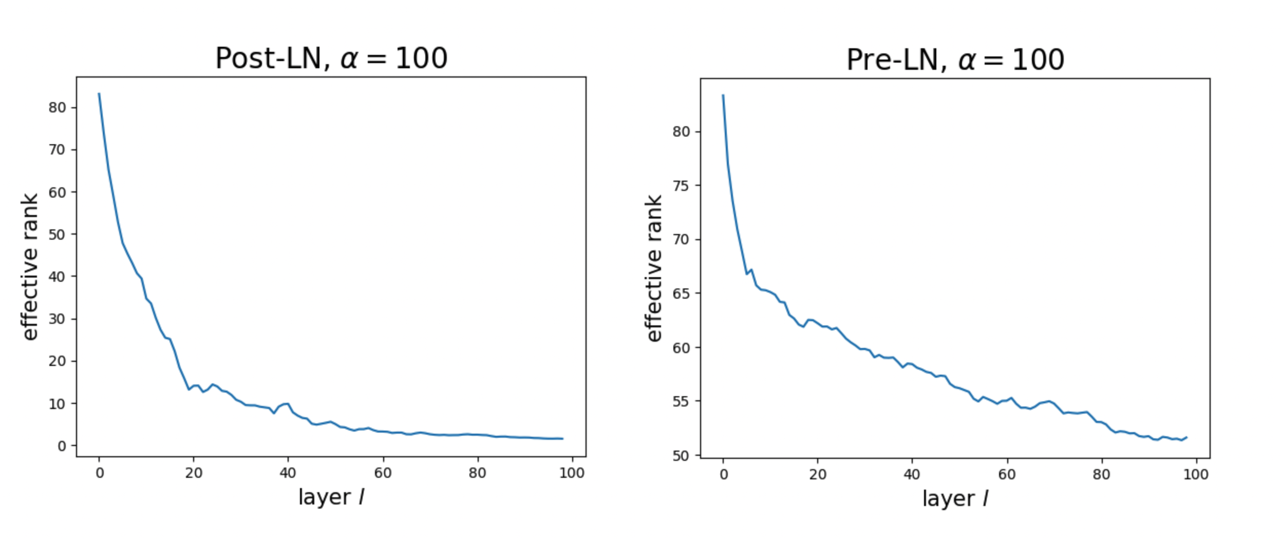
We also compute the effective rank of \(h^l\): we apply PCA to a point cloud of \(h^l\), normalize the singular values into a probability distribution, compute its entropy, and then exponentiate it. The results suggest that Pre-LN maintains representation rank better than Post-LN.

At first, this result confused me, because I had incorrectly equated “representation collapse” with “low representation rank.” In fact, what people usually mean by representation collapse in this context is strong alignment between the representations of consecutive layers, rather than a literal drop in rank.

Questions

Many questions about this toy model remain open:

• Gradient analysis: So far, we have only analyzed forward computations. How do gradients propagate across layers in this setup?
• Many papers (including the Hyper-connection paper) attempt to find a better trade-off between vanishing gradients and representation collapse. Is it possible to eliminate both? Or is there fundamentally no free lunch?

Code

Google Colab notebook available here.

Citation

If you find this article useful, please cite it as:

BibTeX:

@article{liu2026depth-1,
  title={Depth 1 -- Understanding Pre-LN and Post-LN},
  author={Liu, Ziming},
  year={2026},
  month={January},
  url={https://KindXiaoming.github.io/blog/2026/depth-1/}
}