Bigram 4 -- On the difficulty of spatial map emergence

Author: Ziming Liu (刘子鸣)

Motivation

In two previous posts (bigram-1 and bigram-2), we studied a toy task—random walk on a circle. We showed that standard embeddings fail to learn the circular structure underlying the task. This raises a natural question: why is it hard for a spatial map to emerge?

In this article, we deliberately construct a network that can perform the task perfectly when its weights are set appropriately, yet still exhibits failure modes when the weights are randomly initialized and trained via gradient descent. We will analyze these failure modes and propose a simple fix.

Problem setup

Dataset
We use the same dataset as in the previous blogs. Suppose there are \(p=10\) points on a circle. Typical trajectories look like

\[[0] \rightarrow [1] \rightarrow [0] \rightarrow [9] \rightarrow [8] \rightarrow [7] \rightarrow [8] \rightarrow [7] \rightarrow \cdots\] \[[2] \rightarrow [1] \rightarrow [2] \rightarrow [3] \rightarrow [4] \rightarrow [5] \rightarrow [4] \rightarrow [3] \rightarrow \cdots\]

Model
We now construct a network that can solve this task perfectly. Suppose there are \(p\) points in total. The \(i^{\rm th}\) point is embedded as
\(E_i = A\bigl(\cos(\tfrac{2\pi i}{p}), \sin(\tfrac{2\pi i}{p})\bigr).\)

To walk clockwise to the neighboring point, we need a rotation matrix with angle \(\theta=\frac{2\pi}{p}\): \(R(\theta)= \begin{pmatrix} \cos\theta & \sin\theta \\ -\sin\theta & \cos\theta \end{pmatrix},\) parameterized as \(W_1\).
To walk counter-clockwise to the neighboring point, we need \(R(-\theta)\), parameterized as \(W_2\).

To read out each location, the unembedding matrix shares the same weights as the embedding matrix. To create a bimodal distribution, we must average two probability distributions (not add two logits; note that this cannot be efficiently simulated by standard layers).

In summary, when embeddings lie on a circle with a large radius \(A\), and when \(W_1\) and \(W_2\) learn the corresponding rotation matrices, the task can be solved perfectly.

Observation: random initialization fails to learn a circle

We set \(n_{\rm embd}=2\) and \(p=29\). We show results from six different random seeds; in none of them does a circular structure emerge.

From bigram-2, we learned that there may exist negative directions in which points that are close in physical space are actually far apart in embedding space. This motivates the following experiments—fixing \(W_1\) and \(W_2\).

Experiment 1

We initialize \(W_1\) and \(W_2\) to simple matrices (corresponding to Euclidean, hyperbolic, and anti-Euclidean geometries) and keep them fixed during training.

First case – \(W_1=W_2=\mathrm{diag}(1,1)\):
A circular structure can be learned for most random seeds. The perplexity (4.15) is still high because a token is closest to itself—the model therefore predicts the most probable next point to be the current point. However, the ground truth is either the left or the right neighbor, leading to high loss.

Second case – \(W_1=W_2=\mathrm{diag}(1,-1)\):
A global circular structure is visible, but it is locally incorrect (pairs of points collapse together), and the numerical order is not clean.

Third case – \(W_1=W_2=\mathrm{diag}(-1,-1)\):

At first glance, a perfect circle seems to emerge. However, upon closer inspection, the ordering is incorrect—for example, 9 is opposite to 8/10 rather than being nearby. Interestingly, the perplexity is lower than in the first case. In fact, the perplexity (2.01) is close to the theoretical optimum of 2. This is because this embedding geometry places a token far from itself, whereas in the first case a token is closest to itself (corresponding to staying in place, which is not allowed by the task).

Experiment 2

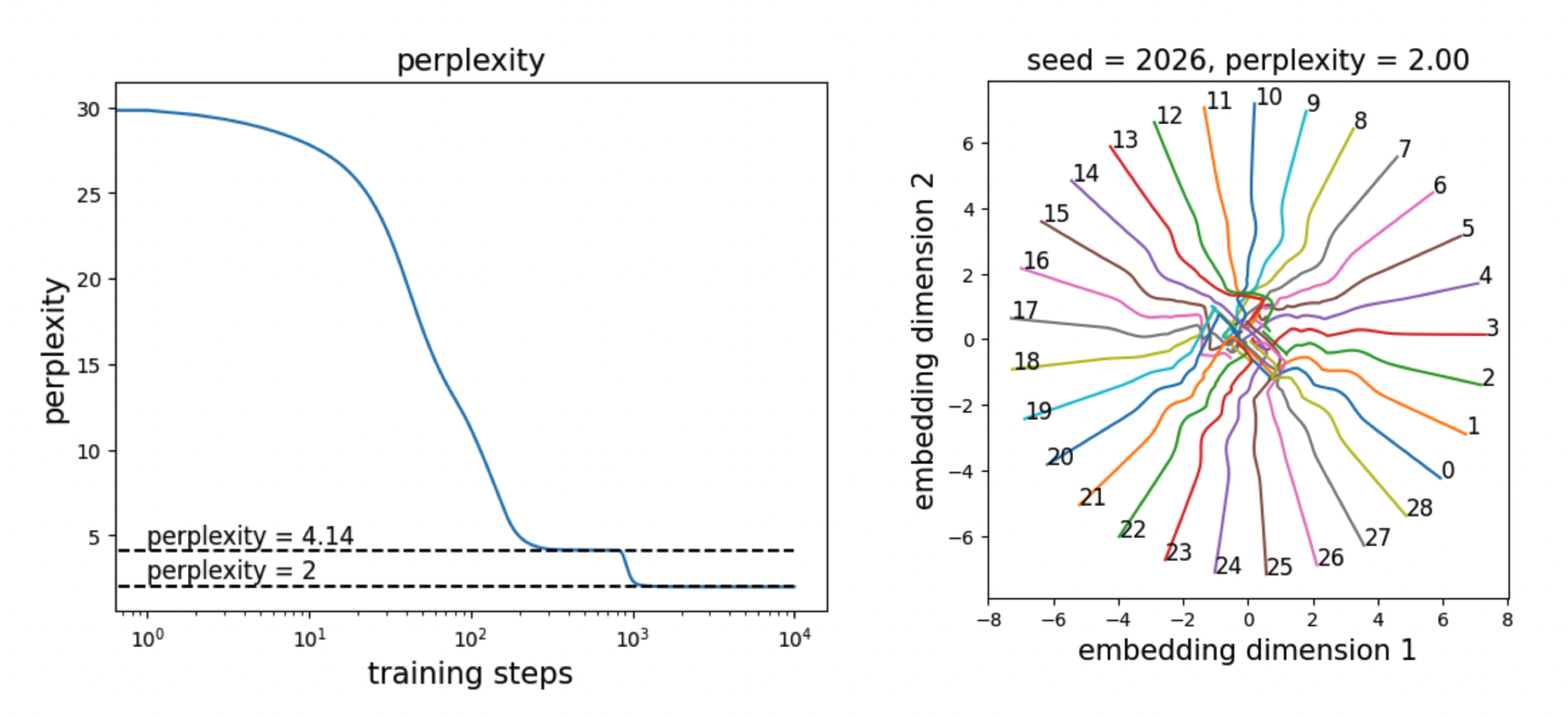
We set \(W_1=W_2=\mathrm{diag}(1,1)\) (injecting small noise to break symmetry) and allow them to be trainable. During training, the perplexity first converges to 4.14 (embeddings evolve while \(W_1/W_2\) remain nearly fixed), and then transitions to 2 (embeddings stabilize while \(W_1/W_2\) evolve).

Comment

When a sequence of tokens is generated by an underlying continuous process, it may be beneficial to initialize projection matrices as the identity, allowing spatial locality to be learned.
Does this initialization trick work for natural language? Not necessarily, for two reasons:
(1) Although one may argue that neural activity (which determines speech) is continuous, the time scales differ—neural activity operates on millisecond scales, whereas natural language unfolds over seconds.
(2) Natural language appears more discrete than continuous. The random-walk dataset is therefore not a good abstraction of language. Instead, we need toy language datasets that capture discrete dependency graphs.
The toy model we studied in this article is non-standard, because it is specifically designed for the random walk task.

Code

Google Colab notebook available here.

Citation

If you find this article useful, please cite it as:

BibTeX:

@article{liu2026bigram-4,
  title={Bigram 4 -- On the difficulty of spatial map emergence},
  author={Liu, Ziming},
  year={2026},
  month={January},
  url={https://KindXiaoming.github.io/blog/2026/bigram-4/}
}