Bigram 3 -- Low Rank Structure

Author: Ziming Liu (刘子鸣)

Motivation

In large language models (LLMs), the embedding dimension is typically much smaller than the vocabulary size, yet models still perform remarkably well. Does this suggest that language itself possesses some kind of low-rank structure?

In this article, we study a Bigram dataset, where each token depends only on the immediately preceding token. We further assume that the (log) transition probability matrix has a low-rank structure. This naturally raises the following question: Is it sufficient for the embedding dimension to match this rank, rather than scaling all the way up to the vocabulary size?

Problem setup

Dataset
Let the vocabulary size be \(V\) and the rank be \(R\). We generate two random matrices \(A\in\mathbb{R}^{V\times R}, \quad B\in\mathbb{R}^{R\times V}.\) Their matrix product \(L = AB/\sqrt{R}\) is a low-rank matrix. The factor \(1/\sqrt{R}\) ensures that the scale of \(L\) is independent of \(R\). Applying a row-wise softmax to \(L\) yields the transition matrix \(P = {\rm Softmax}(L, {\rm dim}=1).\)

From the transition matrix, we can compute the steady-state distribution \(\pi\), which is interpreted as the token frequency (i.e., the unigram distribution). To generate a batch of data, we proceed in two steps:

Step 1: sample the input token from the unigram distribution.
Step 2: sample the output token from the transition matrix, conditioned on the input token.

The best achievable loss \(L_0\) is given by the conditional entropy, averaged over input tokens.

We can introduce additional knobs to control the dataset:

Instead of assuming all \(R\) ranks are equally important, we can assign different weights by inserting a diagonal matrix between \(A\) and \(B\): \(AB \;\to\; A\Lambda B.\)
We can also control the overall scale of the logit matrix. When this scale is large, the dataset becomes more deterministic.

Model
Our model consists only of an Embedding layer and an Unembedding layer, whose weights are not tied. The main quantity of interest in this article is the embedding dimension \(N\).

Observation 1: critical embedding dimension \(N_c\approx R\)

We set \(V=10\) and \(R=3\). We expect that when \(N=N_c=3\), the model can achieve the optimal loss \(L_0\), whereas for \(N<N_c\) the loss should be strictly higher. This is indeed what we observe.

Observation 2: scaling laws in the regime \(N<R\)

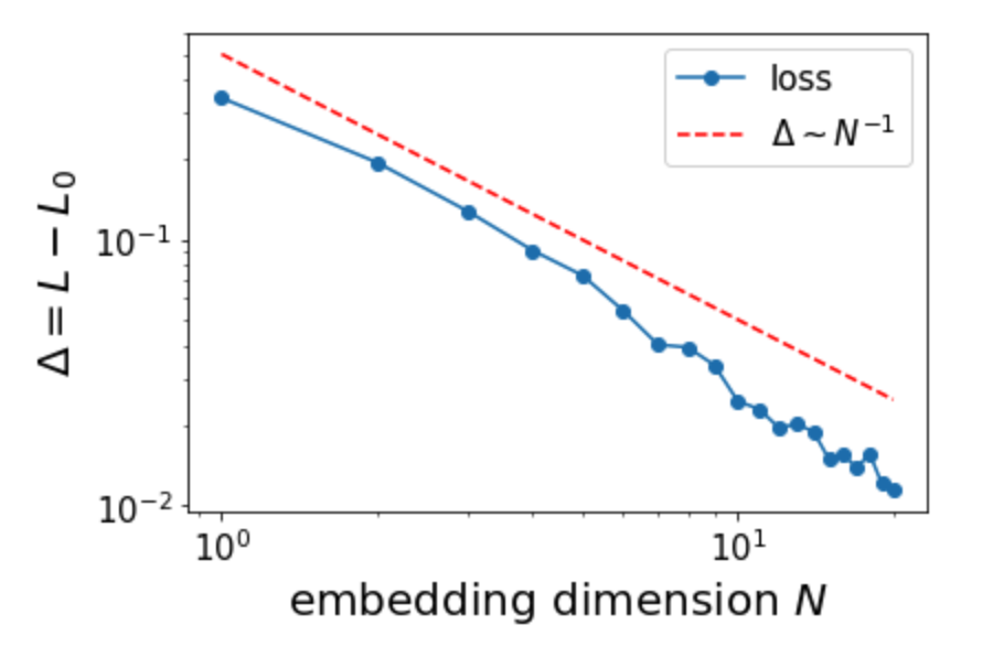
We now set \(V=100\) and \(R=20\), and sweep \(N\) from 1 to 20. Defining the loss gap \(\Delta \equiv L - L_0,\) we find that it closely follows a scaling law \(\Delta \sim N^{-1}.\) This can be viewed as a generalization of the result reported in this paper.

Questions

Many questions about this toy model remain open:

Loss analysis: which token(s) incur the largest loss?
Training dynamics: how do the embeddings evolve during training?
Architecture choices: how do weight sharing, attention, MLPs, and layer normalization affect the results?

Code

Google Colab notebook available here.

Citation

If you find this article useful, please cite it as:

BibTeX:

@article{liu2026bigram-3,
  title={Bigram 3 -- Low Rank Structure},
  author={Liu, Ziming},
  year={2026},
  month={January},
  url={https://KindXiaoming.github.io/blog/2026/bigram-3/}
}