Bigram 2 -- Emergence of Hyperbolic Spaces
Author: Ziming Liu (刘子鸣)
Motivation
In yesterday’s blog post, we studied a simple Markov chain—a random walk on a circle. We found that when the embedding dimension is 2, the model fails to perform the task (even though a circle can, in principle, be perfectly embedded in 2D). However, when the embedding dimension is increased to 4, the model can solve the task perfectly. At the time, we did not understand what the 4D solution was actually doing. This article is an attempt to understand the mechanism behind this 4D algorithm.
Problem setup
Dataset
We use the same dataset as in the previous blog. Suppose there are 10 points on the circle. Typical trajectories look like
Model
The model consists only of an Embedding layer, an Unembedding layer (with tied weights), and a linear layer \(A\) in between. This is equivalent to an Attention layer with context length 1, where \(A = OV\).
When there is no linear layer \(A\) (or equivalently \(A = I\)), the model completely fails to perform this task. In that case, the model most likely repeats the current token, rather than predicting the token to its left or right (we will discuss this more carefully at the end of the article, but for now we take this as a given fact). Therefore, the linear layer \(A\) is necessary.
Observation 1: \(A\) is symmetric, and has negative eigenvalues (hyperbolic directions)
When \(n_{\rm embd} = 4\), the perplexity can go down to 2 (the best achievable perplexity). By directly inspecting the embeddings or their PCA projections, we fail to observe any obvious pattern.

However, we notice that the linear matrix \(A\) is close to a symmetric matrix:
\[A = \begin{pmatrix} -3.3250 & -2.0423 & 2.0838 & -3.5954 \\ -2.0604 & -3.2431 & -2.8658 & 2.8647 \\ 2.0648 & -2.8236 & -2.5492 & -2.8768 \\ -3.5372 & 2.7750 & -2.8383 & -1.5314 \\ \end{pmatrix}\]A symmetric matrix can be diagonalized over the real numbers. The four eigenvalues consist of two positive and two negative values: \([-5.88, -5.41, 5.42, 6.40],\) all of comparable magnitude. It is therefore more natural to project the embeddings onto the eigen-directions:

We find that the two negative-eigenvalue directions are highly oscillatory (adjacent tokens have opposite signs), whereas the two positive-eigenvalue directions are much smoother (adjacent tokens have similar values).
Consider an input token \(m\) with embedding \(E_m\). Its logit for token \(n\) is given by \(E_n^T A E_m\), which is a quadratic form. Along positive eigen-directions, the logit is lower if two embeddings have opposite signs. In contrast, along negative eigen-directions, the logit is higher if two embeddings have opposite signs. The coexistence of positive and negative eigenvalues effectively turns the embedding space into a hyperbolic space, which can strongly conflict with our Euclidean geometric intuition.
More formally, for two vectors \(x, y\) in this space, their similarity can be written as \(L(i,j) \sim -x_1 y_1 - x_2 y_2 + x_3 y_3 + x_4 y_4.\)
For nearby tokens, we want the similarity to be large. This can be achieved by having opposite signs along the negative eigen-directions, and the same signs (similar values) along the positive eigen-directions. This mixed strategy makes interpretation difficult: although tokens \(i\) and \(i+1\) correspond to nearby points on the circle, they are not necessarily close in the embedding space, because the negative eigen-directions actively push them as far apart as possible.
Two remarks are in order:
\(A\) is not necessarily symmetric.
In our case, \(A\) is symmetric because the Markov process we study is reversible. In general, \(A\) need not be symmetric, and it is unclear how to deal with a non-symmetric \(A\), where the left and right eigenspaces are no longer aligned.
More to understand.
So far, we have established that the embedding space is hyperbolic, which is already a somewhat surprising result with potentially significant implications for interpretability. However, many details are still missing, in particular how the tokens are arranged quantitatively within this hyperbolic space.
Observation 2: Geometry matters
We find that \(n_{\rm embd} = 4\) works (i.e., the perplexity converges to 2) only for lucky random seeds. For unlucky random seeds, the perplexity instead converges to around 2.13. What distinguishes these cases? We observe that the geometry—specifically, the number of negative directions—is highly correlated with performance.
When there are 2 or 3 negative directions, the optimal perplexity is achievable. With only 1 negative direction, optimization appears to get stuck in a local minimum.
| Random Seed | Perplexity | Eigenvalues | Negative Number |
|---|---|---|---|
| 0 | 2.13 | -7.6, 5.6, 5.7, 6.7 | 1 |
| 1 | 2.13 | -7.7, 5.1, 6.1, 6.2 | 1 |
| 2 | 2.13 | -7.2, 5.7, 6.4, 6.5 | 1 |
| 3 | 2.00 | -6.1, -5.8, -4.4, 5.6 | 3 |
| 4 | 2.00 | -5.9, -5.4, 5.4, 6.4 | 2 |
| 5 | 2.00 | -6.7, -6.0, -5.7, 6.5 | 3 |
| 6 | 2.10 | -7.0, 5.3, 5.7, 6.2 | 1 |
| 7 | 2.00 | -5.7, -5.2, -4.9, 5.4 | 3 |
| 8 | 2.00 | -5.8, -4.8, 4.6, 5.9 | 2 |
| 9 | 2.10 | -7.0, 5.1, 6.1, 7.1 | 1 |
| 42 | 2.10 | -7.1, 6.0, 6.3, 6.8 | 1 |
| 2026 | 2.00 | -5.1, -4.8, 4.7, 5.8 | 2 |
Sanity check: why do we need \(A\)?
When we remove \(A\) or set \(A = I\), the perplexity remains far above 2, regardless of how large the embedding dimension is. When \(A = I\) (so the embedding space is purely Euclidean), an input token has no mechanism to “un-attend” to itself. In contrast, a negative eigen-direction can serve precisely this un-attention role, a mechanism also explored in Sparse-attention-2. As a result, \(A\) is essential for performing the random-walk task.
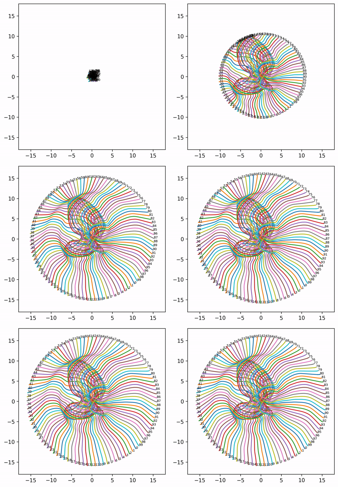
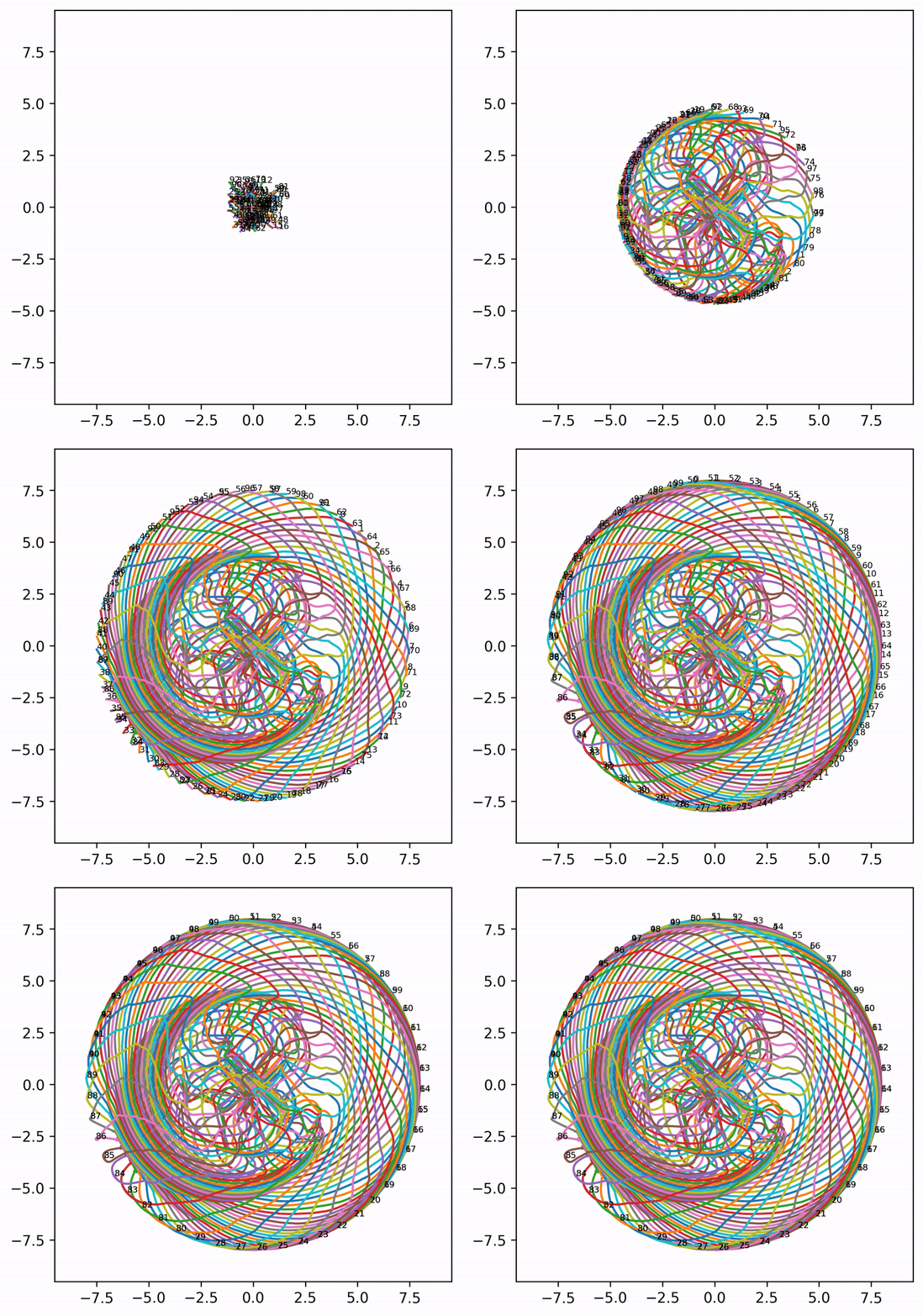
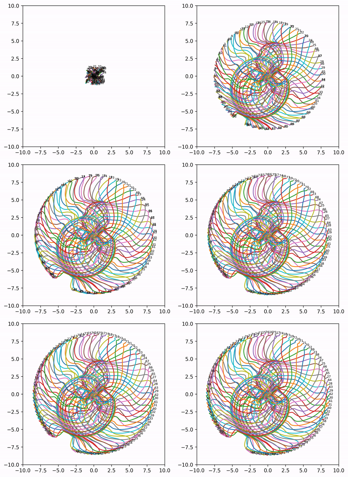
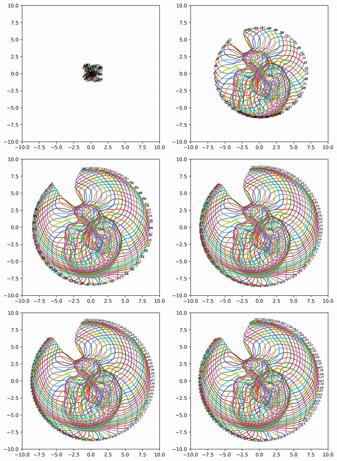
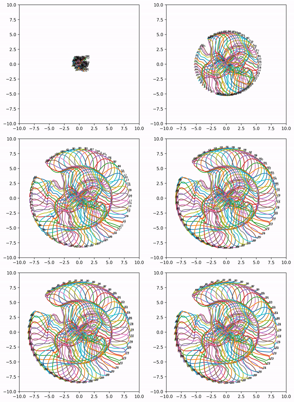
That said, when \(A = I\) (i.e., attention is completely removed) and \(n_{\rm embd} = 2\), the embeddings can evolve into extremely wild (and aesthetically pleasing) patterns. Even though these patterns may not shed much light on what is really happening in language models, it is pure pleasure to watch the resulting animations.
Seed = 0
Seed = 1
Seed = 4
Seed = 6
Seed = 9
Code
Google Colab notebook available here.
Citation
If you find this article useful, please cite it as:
BibTeX:
@article{liu2026bigram-2,
  title={Bigram 2 -- Emergence of Hyperbolic Spaces},
  author={Liu, Ziming},
  year={2026},
  month={January},
  url={https://KindXiaoming.github.io/blog/2026/bigram-2/}
}
Enjoy Reading This Article?
Here are some more articles you might like to read next: